Recursion is a powerful tool that allows you to solve complex problems in a simple and elegant way. In this guide, we will explore the fundamentals of recursion, including practical examples that demonstrate how to efficiently solve problems involving repeated subproblems. Topics such as tail recursion, mutual recursion, and common pitfalls to avoid when using recursion in algorithms are explored in detail.

Recursion is a powerful problem-solving technique. Its origins can be traced back to the early 20th century, when mathematicians like Alonzo Church and Kurt Gödel explored recursive functions in the context of formal logic and computation. Church’s development of lambda calculus in the 1930s laid the foundation for recursion as a method to define functions that reference themselves. These theoretical advancements not only influenced the field of mathematics but also provided the groundwork for modern computer science, where recursion became a fundamental tool for solving complex problems.

From a mathematical perspective, recursion is closely related to the principle of mathematical induction. Just as induction proves the correctness of statements for all natural numbers by establishing a base case and an inductive step, recursion operates similarly. We solve a problem by breaking it down into smaller subproblems, and the solution is built upon the base case.

In a recursive algorithm, the base case provides the stopping condition, while the recursive step ensures that each recursive call progresses toward this base case. To mathematically prove the correctness of a recursive algorithm, we follow the structure of an induction proof:

• Base case: Prove that the algorithm works for the smallest instance of the problem.
• Recursive step: Assume the algorithm works for smaller instances and prove it works for the current instance.

Let’s take the recursive factorial function as an example:

To prove this function is correct using mathematical induction, we follow these steps:

• Base case: For $n = 0$, the function returns 1, which is correct since $0! = 1$ by definition.
• Inductive hypothesis: Assume the function works for $n = k$, i.e., $k! = k \times (k-1)!$.
• Inductive step: Prove that the function works for $n = k+1$. According to the definition of factorial, $(k+1)! = (k+1) \times k!$, which the function computes correctly by calling $\text{factorial}(k)$. Thus, by the inductive hypothesis, the function is correct for $n = k+1$.

Therefore, by induction, the recursive factorial function is correct for all $n \geq 0$.

Beyond the ease of mathematical proof, which, by the way, is your problem, recursive code stands out for being clear and intuitive, especially for problems with repetitive structures such as tree traversal, maze solving, and calculating mathematical series.

Many problems are naturally defined in a recursive manner. For example, the mathematical definition of the Fibonacci Sequence or the structure of binary trees are inherently recursive. In these cases, the recursive solution will be simpler, more straightforward, and likely more efficient.

Often, the recursive solution is more concise and requires fewer lines of code compared to the iterative solution. Fewer lines, fewer errors, easier to read and understand. Sounds good.

Finally, recursion is an almost ideal approach for applying divide-and-conquer techniques. Since Julius Caesar, we know it is easier to divide and conquer. In this case, a problem is divided into subproblems, solved individually, and then combined to form the final solution. Classic academic examples of these techniques include sorting algorithms like quicksort and mergesort.

The sweet reader might have raised her eyebrows. This is where recursion and Dynamic Programming touch, not subtly and delicately, like a lover’s caress on the beloved’s face. But with the decisiveness and impact of Mike Tyson’s glove on the opponent’s chin. The division of the main problem into subproblems is the fundamental essence of both recursion and Dynamic Programming.

Dynamic Programming and recursion are related; both involve solving problems by breaking a problem into smaller problems. However, while recursion solves the smaller problems without considering the computational cost of repeated calls, Dynamic Programming optimizes these solutions by storing and reusing previously obtained results.A classic illustration of recursion is the calculation of the nth term in the Fibonacci Sequence, as depicted in Flowchart 1.

Flowchart 1 - Recursive Fibonacci nth algorithm

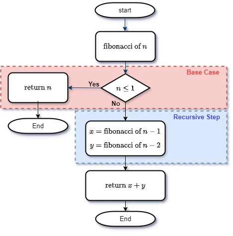
The Flowchart 1 represents a function for calculating the nth number of the Fibonacci Sequence, for all $n \geq 0$ as the desired number. In Flowchart 1 we have:

• Base Case: The base case is the condition that terminates the recursion. For the Fibonacci Sequence, the base cases are for $n = 0$ and $n = 1$:

  • When $n = 0$, the function returns $0$.
  • When $n = 1$, the function returns $1$.

• Recursive Step: The recursive step is the part of the function that calls itself to solve smaller subproblems. In the Fibonacci Sequence, each number is the sum of the two preceding ones: $F(n) = F(n - 1) + F(n - 2)$ which leads to a representation of the base cases as: $F(0) = 0$ and $F(1) = 1$

When the function receives a value $n$:

• Base Case: It checks if $n$ is 0 or 1. If so, it returns $n$.
• Recursive Step: If $n$ is greater than 1, the function calls itself twice: Once with $n - 1$ and once with $n - 2$. The sum of these two results is returned.

To illustrate, let’s calculate the 5th Fibonacci number.

Example 1: Recursion

1. fibonacci(5) calls fibonacci(4) and fibonacci(3)
2. fibonacci(4) calls fibonacci(3) and fibonacci(2)
3. fibonacci(3) calls fibonacci(2) and fibonacci(1)
4. fibonacci(2) calls fibonacci(1) and fibonacci(0)
5. fibonacci(1) returns 1
6. fibonacci(0) returns 0
7. fibonacci(2) returns $1 + 0 = 1$
8. fibonacci(3) returns $1 + 1 = 2$
9. fibonacci(2) returns 1 (recalculated)
10. fibonacci(4) returns $2 + 1 = 3$
11. fibonacci(3) returns 2 (recalculated)
12. fibonacci(5) returns $3 + 2 = 5$

Thus, fibonacci(5) returns $5$. The function breaks down recursively until it reaches the base cases, then combines the results to produce the final value.

And we can write it in Python, using Python as a kind of pseudocode, as:

def fibonacci(n):
    if n <= 1:
        return n
    else:
        return fibonacci(n-1) + fibonacci(n-2)

Code Fragment 1 - Recursive Fibonacci Function for the nth Term

In Code Fragment 1, the fibonacci function calls itself to calculate the preceding terms of the Fibonacci Sequence. Note that for each desired value, we have to go through all the others. This is an example of correct and straightforward recursion and, in this specific case, very efficient. This implementation is clear and mirrors the mathematical definition of the Fibonacci sequence. However, it has some efficiency issues for larger values of $n$. Let’s take a look at this efficiency issue more carefully later.

Calculate the Number of Recursive Calls

To quantify the number of times the fibonacci function is called to calculate the 5th number in the Fibonacci Sequence, we can analyze the recursive call tree. “Let’s enumerate all function calls, accounting for duplicates.

Using the previous example and counting the calls:

1. ` fibonacci(1)``fibonacci(5) `
2. fibonacci(4) + fibonacci(3)
3. fibonacci(3) + fibonacci(2) + fibonacci(2) + fibonacci(1)
4. fibonacci(2) + fibonacci(1) + fibonacci(1) + fibonacci(0) + fibonacci(1) + fibonacci(0)
5. fibonacci(1) + fibonacci(0)

Counting all the calls, we have:

• fibonacci(5): 1 call
• fibonacci(4): 1 call
• fibonacci(3): 2 calls
• fibonacci(2): 3 calls
• fibonacci(1): 5 calls
• fibonacci(0): 3 calls

Total: $15$ calls. Therefore, the fibonacci(n) function is called $15$ times to calculate fibonacci(5).

To understand the computational cost of the recursive Fibonacci function, let’s analyze the number of function calls made for a given input $n$. We can express this using the following recurrence relation:

where:

• $T(n)$ represents the total number of calls to the fibonacci(n) function.
• $T(n-1)$ represents the number of calls made when calculating fibonacci(n-1).
• $T(n-2)$ represents the number of calls made when calculating fibonacci(n-2).
• The $+ 1$ term accounts for the current call to the fibonacci(n) function itself.

The base cases for this recurrence relation are:

• $T(0) = 1$
• $T(1) = 1$

These base cases indicate that calculating fibonacci(0) or fibonacci(1) requires a single function call.

To illustrate the formula $T(n) = T(n-1) + T(n-2) + 1$ with $n = 10$, we can calculate the number of recursive calls $T(10)$. Let’s start with the base values $T(0)$ and $T(1)$, and then calculate the subsequent values up to $T(10)$. Therefore we will have:

Therefore, $T(10) = 177$.

Each value of $T(n)$ represents the number of recursive calls to compute fibonacci(n) using the formula $T(n) = T(n-1) + T(n-2) + 1$. If everything is going well, at this point the esteemed reader must be thinking about creating a recursive function to count how many times the fibonacci(n) function will be called. But let’s try to avoid this recursion of recursions in recursions to keep our fragile sanity.

The formula $T(n) = T(n-1) + T(n-2) + 1$ can be used to build a recursion tree, as we can see in Figure 1, and sum the total number of recursive calls. However, for large values of $n$, this can become inefficient. A more efficient approach is to use Dynamic Programming to calculate and store the number of recursive calls, avoiding duplicate calls.

_Figure 1 - Recursive Tree for Fibonacci 5*{: class=”legend”}

Space and Time Efficiency

The fibonacci(n) function employs a straightforward recursive approach to calculate Fibonacci numbers. Let’s analyze its time and space complexity…

Recursion became a central tool in programming with the advent of languages like Lisp in the 1950s, which embraced recursion as a core principle for defining functions. The simplicity and elegance of recursion made it an ideal method for expressing problems like the Fibonacci sequence. In modern functional programming languages, such as Haskell, recursion continues to play a vital role in solving complex problems through elegant, concise code.

To understand the time complexity, consider the frequency of function calls. Each call to fibonacci(n) results in two more calls: fibonacci(n-1) and fibonacci(n-2). This branching continues until we reach the base cases.

Imagine this process as a tree, as we saw earlier:

• The root is fibonacci(n).
• The next level has two calls: fibonacci(n-1) and fibonacci(n-2).
• The level after that has four calls, and so on.

Each level of the tree results in a doubling of calls. If we keep doubling for each level until we reach the base case, we end up with about $2^n$ calls. This exponential growth results in a time complexity of O(2^n), an exponential increase. This is highly inefficient as the number of calls grows exponentially with larger values of $n$.

The space complexity depends on how deep the recursion goes. Every time the function calls itself, it adds a new frame to the call stack.

• The maximum depth of recursion is $n$ levels (from fibonacci(n) down to fibonacci(0) or fibonacci(1)).

Therefore, the space complexity is $O(n)$ where $n$ is the maximum depth of the call stack, as the stack grows linearly with $n$.

In short, the recursive fibonacci function is simple but inefficient for large $n$ due to its exponential time complexity. This is where Dynamic Programming becomes useful. Dynamic Programming optimizes the recursive solution by storing the results of subproblems, thereby avoiding redundant calculations.

By using Dynamic Programming, we can optimize the recursive Fibonacci algorithm by storing the results of subproblems in a table. This eliminates redundant calculations and transforms the recurrence relation into:

This results in a linear time complexity of:

Thus, using memoization or dynamic programming, we reduce the time complexity from $O(2^n)$ to $O(n)$, making the algorithm much more efficient for large values of $n$.

The concept of recursion, first explored in the realm of mathematical logic by pioneers like Alonzo Church and Kurt Gödel, has evolved into a powerful tool for modern computing. From its theoretical roots in the 1930s to its widespread adoption in programming languages today, recursion remains a cornerstone of both theoretical and practical problem-solving.