
Competitive programming in C++ - Techniques and Insights

In this comprehensive guide, we delve into the world of Competitive Programming with C++. Learn the core principles of Competitive Programming, explore various algorithmic examples, and understand performance differences through detailed code comparisons. Perfect for developers looking to optimize their coding skills and boost algorithm efficiency.
1. Introduction
C++ remains one of the most popular languages in competitive programming due to its performance, flexibility, and rich standard library. Mastering efficient C++ techniques is crucial for success in programming contests, where solving complex problems under strict time and memory constraints is the norm. This guide delves into advanced C++ programming strategies, focusing on Dynamic Programming - a powerful algorithmic paradigm that solves complex problems by breaking them down into simpler subproblems. By optimizing input/output operations, leveraging modern C++ features, and utilizing efficient data structures and algorithms, we’ll explore how to apply Dynamic Programming techniques to tackle a wide range of computational challenges.
For instance, one common optimization in competitive programming is to speed up input/output operations. By default, C++ performs synchronized I/O with C’s standard I/O libraries, which can be slower. A simple trick to improve I/O speed is disabling this synchronization:
    std::ios_base::sync_with_stdio(false);
    cin.tie(nullptr);
This small change can make a significant difference when dealing with large input datasets. Throughout this guide, we will cover similar techniques, along with advanced input/output operations, efficient use of data structures like arrays and vectors, and modern C++20 features that help streamline your code. You’ll also learn optimizations to minimize overhead and how to effectively leverage STL containers and algorithms to improve both runtime performance and code readability. Whether you are solving large-scale data processing problems or optimizing for time-critical solutions, the strategies in this guide will equip you to perform at a high level in programming contests.
We begin by exploring various methods to strengthen file I/O and array handling, which are fundamental to processing large datasets quickly. The guide then progresses through different looping constructs, from basic for and while loops to more advanced C++20 features like range-based for loops with views and parallel execution policies. We also cover important optimizations such as minimizing typing overhead, utilizing the Standard Template Library (STL) effectively, and employing memory-efficient techniques like std::span. Throughout this journey, we’ll focus on how these C++ features and optimizations can be applied to implement efficient Dynamic Programming solutions, enabling you to solve complex algorithmic puzzles with improved performance and reduced memory usage.
C++ is particularly effective for solving a wide range of problems in competitive programming. Some common types of problems where C++ excels include:
- Array Manipulation: Efficiently processing and querying large arrays or sequences.
- Graph Algorithms: Implementing complex graph traversals and shortest path algorithms.
- String Processing: Handling string matching, parsing, and manipulation tasks.
- Data Structures: Implementing and utilizing advanced data structures like segment trees or Fenwick trees.
- Computational Geometry: Solving geometric problems with high precision and efficiency.
These problem types demonstrate how C++’s performance and rich standard library can be leveraged to create optimal solutions in competitive programming scenarios.
By mastering these C++20 techniques, you’ll be well-equipped to tackle a wide range of competitive programming challenges. Whether you’re dealing with large-scale data processing, intricate algorithmic puzzles, or time-critical optimizations, the strategies outlined in this guide will provide you with the tools to write faster, more efficient code. This knowledge not only boosts your performance in competitions but also deepens your understanding of C++ and algorithmic thinking, skills that are valuable beyond the competitive arena.
2. C++ Competitive Programming Hacks
In this section, we’ll cover essential tips and tricks that will help you improve your efficiency and performance in competitive programming using C++. From mastering typing speed to reducing code verbosity and handling complexity, each aspect plays a crucial role in gaining a competitive edge.
C++ is known for its speed and flexibility, but using it effectively requires a deep understanding of both the language and the common pitfalls that arise in competitive programmings. The goal here is to help you streamline your coding process, minimize errors, and ensure that your solutions run as efficiently as possible.
We’ll break down these tips into the following areas:
- Typing Efficiency: How to type faster and more accurately, which can save you valuable time during competitive programming.
- Code Reduction Techniques: Ways to reduce code size without sacrificing clarity or correctness, using C++ features like the Standard Template Library (STL).
- Managing Complexity: Strategies to handle the time and space complexity of algorithms, ensuring that your solutions scale efficiently with larger inputs.
By applying these hacks, you’ll be better equipped to tackle the challenges of competitive programming with C++ and improve your overall performance. Keep in mind that the code and techniques discussed here are optimized specifically for competitive programming environments, where the code is written for single-use and will not be maintained or reused. These approaches may not be suitable for professional development, where code readability, maintainability, and long-term reliability are critical.
2.1 Typing Tips
If you don’t type quickly, you should invest at least two hours per week on the website: https://www.speedcoder.net. Once you have completed the basic course, select the C++ lessons and practice regularly. Time is crucial in competitive programming, and slow typing can be disastrous.
To expand on this, efficient typing isn’t just about speed; it’s about reducing errors and maintaining a steady flow of code. When you’re in a competitive programming, every second matters. Correcting frequent typos or having to look at your keyboard will significantly slow down your progress. Touch typing—knowing the layout of the keyboard and typing without looking—becomes a vital skill.
2.2 Why Typing Speed Matters
In a typical programming competitive programming, you’ll have to solve several problems within a fixed time frame. Faster typing allows you to focus more on problem-solving rather than struggling to input the code. However, typing speed without accuracy is meaningless. Accurate and fast typing ensures that once you have the solution, you can implement it efficiently.
Typing slow or with many errors leads to:
- Lost time correcting mistakes
- Distractions from your problem-solving process
- Higher risk of failing to complete solutions on time
You should aim for a typing speed of at least 60 words per minute (WPM) with high accuracy. On platforms like https://www.speedcoder.net, you can practice typing specific code syntax, which is more effective for programmers compared to general typing lessons. For example, learning C++ or Python shortcuts helps improve your typing speed in actual coding scenarios.
\[\begin{align*} \text{Time spent fixing errors} + \text{Time lost from slow typing} \\ = \text{Lower overall performance in competitive programming} \end{align*}\]2.3 Advanced Typing Techniques for Programmers
Here are some additional tips to improve your typing for competitive programming:
- Use IDE shortcuts: 1. Use IDE shortcuts: Learn keyboard shortcuts for your favorite Integrated Development Environment (IDE). Navigating and editing code using shortcuts reduces time spent moving between mouse and keyboard. In the case of ICPC contests, the IDE provided will typically be Eclipse, so it’s crucial to familiarize yourself with its shortcuts and navigation to maximize efficiency during the competitive programming. However, it’s important to note that the choice of IDE may change, and contestants should always check the specific rules and environments for each competition.
- Focus on frequent patterns: As you practice, focus on typing patterns you use frequently, such as loops, if-else conditions, and function declarations. Automating these patterns in your muscle memory will save valuable time.
- Practice algorithm templates: Some problems require similar algorithms, such as dynamic programming, sorting, or tree traversal. By practicing typing these algorithms regularly, you’ll be able to quickly implement them during competitive programmings.
In competitive programming, every second counts, and being proficient with your typing can give you a significant advantage.
2.4 Typing Less in Competitive Programming
In competitive programming, time is a critical resource. Therefore, optimizing typing speed and avoiding repetitive code can make a significant difference. Below, we will discuss strategies to minimize typing when working with std::vector during competitive programmings, where access to the internet or pre-prepared code snippets may be restricted.
2.4.1. Using #define for std::vector Abbreviations
We can use #define to create short aliases for common vector types. This is particularly useful when you need to declare multiple vectors throughout the code.
#define VI std::vector<int>
#define VVI std::vector<std::vector<int>>
#define VS std::vector<std::string>
With these definitions, declaring vectors becomes much faster:
VI numbers;  // std::vector<int> numbers;
VVI matrix;  // std::vector<std::vector<int>> matrix;
VS words;    // std::vector<std::string> words;
However, it’s important to note that in larger, professional projects, using #define for type aliases is generally discouraged because it does not respect C++ scoping rules and can lead to unexpected behavior during debugging. In competitive programming, where speed is essential, this technique can be useful, but it should be avoided in long-term or collaborative codebases.
2.4.2. Predefined Utility Functions
Another effective strategy is to define utility functions that you can reuse for common vector operations, such as reading from input, printing, or performing operations like sorting or summing elements.
Reading Vectors:
#define FAST_IO std::ios::sync_with_stdio(false); std::cin.tie(nullptr);

void read_vector(VI& vec, int n) {
    if (n > 0) vec.reserve(static_cast<size_t>(n));
    for (int i = 0; i < n; ++i) {
        int x;
        std::cin >> x;
        vec.push_back(x);
    }
}
With the read_vector function, you can quickly read a vector of n elements:
FAST_IO

VI numbers;
read_vector(numbers, n);
Printing Vectors:
void print_vector(const VI& vec) {
    for (const int& x : vec) {
        std::cout << x << " ";
    }
    std::cout << "\n";
}
This function allows you to easily print the contents of a vector:
print_vector(numbers);
2.4.3. Predefining Common Operations
If you know that certain operations, such as sorting or summing elements, are frequent in a competitive programming, consider defining these operations at the beginning of the code.
Sorting Vectors:
#define SORT_VECTOR(vec) std::sort(vec.begin(), vec.end())
You can then sort any vector quickly:
SORT_VECTOR(numbers);
Summing Elements:
int sum_vector(const VI& vec) {
    return std::accumulate(vec.begin(), vec.end(), 0);
}
To calculate the sum of a vector’s elements:
int total = sum_vector(numbers);
2.4.4. Using Lambda Functions
In C++11 and later versions, lambda functions can be a quick and concise way to define operations inline for vectors:
auto print_square = [](const VI& vec) {
    for (int x : vec) {
        std::cout << x * x << " ";
    }
    std::cout << "\n";
};
These inline functions can be defined and used without the need to write complete functions:
print_square(numbers);
While lambda functions can be very useful for quick, one-off operations, it’s important to note that excessive use of lambdas, especially complex ones, can make code harder to read and maintain. In competitive programming, where code clarity might be sacrificed for speed, this may be less of a concern. However, it’s a good practice to be mindful of code readability, especially when debugging complex algorithms.
2.4.5 Prefer Not to Use #define
Another way to reduce typing time is by using typedef or using to create abbreviations for frequently used vector types:
typedef std::vector<int> VI;
typedef std::vector<std::vector<int>> VVI;
using VS = std::vector<std::string>;
In many cases, the use of #define can be replaced with more modern and safe C++ constructs like using, typedef, or constexpr. #define does not respect scoping rules and does not offer type checking, which can lead to unintended behavior. Using typedef or using provides better type safety and integrates smoothly with the C++ type system, making the code more predictable and easier to debug.
-
Replacing
#definewith Type AliasesFor example:
#define VI std::vector<int>
#define VVI std::vector<std::vector<int>>
#define VS std::vector<std::string>
Can be replaced with
usingortypedefto create type aliases:using VI = std::vector<int>; using VVI = std::vector<std::vector<int>>; using VS = std::vector<std::string>; // Or using typedef (more common in C++98/C++03) typedef std::vector<int> VI; typedef std::vector<std::vector<int>> VVI; typedef std::vector<std::string> VS;usingandtypedefare preferred because they respect C++ scoping rules and offer better support for debugging, making the code more secure and readable. -
Replacing
#definewith Constants -
Using
constexprin FunctionsIf you have macros that perform calculations, you can replace them with
constexprfunctions:Example:
#define SQUARE(x) ((x) * (x))Can be replaced with:
constexpr int square(int x) { return x * x; }constexprfunctions provide type safety, avoid unexpected side effects, and allow the compiler to evaluate the expression at compile-time, resulting in more efficient and safer code.
For competitive programming, using #define might seem like the fastest way to reduce typing and speed up coding. However, using typedef or using is generally more efficient because it avoids potential issues with macros and integrates better with the compiler. While reducing variable names or abbreviating functions might save time during a competitive programming, remember that in professional code, clarity and maintainability are far more important. Therefore, avoid using shortened names and unsafe constructs like #define in production code, libraries, or larger projects.
3. Optimizing File I/O in C++ for competitive programmings
In many competitive programming contests, especially those involving large datasets, the program is required to read input from a file that can be very large. For this reason, it is crucial to optimize how files are read. Efficient file handling can make the difference between a solution that completes within the time limits and one that does not. Implementing techniques to speed up file I/O is indispensable for handling such cases effectively.
3.1 Disabling I/O Synchronization
To improve the performance of input/output (I/O) operations, we disable the synchronization between the standard C and C++ I/O libraries:
std::ios::sync_with_stdio(false);
std::cin.tie(nullptr);
- The function
std::ios::sync_with_stdio(false)disables the synchronization of the C++ streams with the C streams, allowing the program to perform I/O operations more quickly. std::cin.tie(nullptr)detaches the input stream (std::cin) from the output stream (std::cout), preventing automatic flushes that can cause delays.
When we disable synchronization with std::ios::sync_with_stdio(false);, the program benefits from better performance in I/O operations since it no longer needs to synchronize the C++ input/output functions (std::cin, std::cout) with the C functions (scanf, printf).
This synchronization, when enabled, introduces overhead because the system ensures that both libraries can be used simultaneously without conflict. By removing this synchronization, we eliminate that overhead, allowing I/O operations to be processed more directly and faster.
This optimization is particularly beneficial in programs that perform a large number of read and write operations, such as when processing large amounts of data from files. Additionally, by using std::cin.tie(nullptr);, we prevent std::cout from being automatically flushed before each input operation, avoiding another form of latency that could impact performance in I/O-heavy contexts.
3.2 Command Line Argument Checking
Before proceeding with execution, the code checks if exactly one argument was passed through the command line, which represents the name of the file to be read:
if (argc != 2) {
    std::cerr << "Usage: " << argv[0] << " <file_name>\n";
    return 1;
}
argcis the number of arguments passed to the program, including the name of the executable.argvis an array of strings containing the arguments.- If the number of arguments is not 2, the program prints an error message and exits with
return 1, indicating failure.
3.3 Opening and Verifying the File
The code attempts to open the specified file and checks whether the opening was successful:
std::ifstream file(argv[1]);
if (!file) {
    std::cerr << "Error opening file: " << argv[1] << "\n";
    return 1;
}
std::ifstream file(argv[1]);attempts to open the file for reading.- If
fileis not in a valid state (i.e., the file couldn’t be opened), an error message is displayed, and the program terminates.
While good practice in general software development, is usually unnecessary in competitive programming contests. Instead, you can often assume the file exists and start reading from it directly. This saves valuable coding time and simplifies your solution.
4. Introduction to File I/O in C++
In C++, file input and output (I/O) operations are handled through classes provided by the <fstream> library. The three main classes used for this purpose are std::ifstream, std::ofstream, and std::fstream. Each of these classes is specialized for different types of I/O operations.
4.1 std::ifstream: File Reading
The std::ifstream class (input file stream) is used exclusively for reading files. It inherits from std::istream, the base class for all input operations in C++.
4.1.1 Opening Files for Reading
In our code, we use std::ifstream to open a text file and read its contents:
std::ifstream file(argv[1]);
std::ifstream file(argv[1]);: Tries to open the file whose name is passed as a command-line argument. If the file cannot be opened, thefilestream will be invalid.
Off course we can use std::ifstream to read files from command line:
#include <fstream>
#include <iostream>
#include <string>

int main(int argc, char* argv[]) {
    if (argc != 2) {
        std::cerr << "Usage: " << argv[0] << " <filename>\n";
        return 1;
    }

    // Abre o arquivo apenas para leitura
    std::ifstream file(argv[1]);

    if (!file.is_open()) {
        std::cerr << "Error: Could not open the file " << argv[1] << "\n";
        return 1;
    }

    std::string line;

    // Lê o conteúdo do arquivo linha por linha e exibe no console
    std::cout << "Contents of the file:\n";
    while (std::getline(file, line)) {
        std::cout << line << "\n";
    }

    file.close();
    return 0;
}
4.1.2 Verifying File Opening
After attempting to open the file, it’s crucial to check whether the opening was successful:
if (!file) {
    std::cerr << "Error opening file: " << argv[1] << "\n";
    return 1;
}
if (!file): Checks if thefilestream is in an invalid state (which indicates the file was not opened correctly). If the file can’t be opened, an error message is displayed, and the program exits.
Again, in competitive programmings, the input file will most often be handled by an automated testing system, so you probably won’t need to check whether the file opened correctly or not.
4.1.3 File Reading
Once the file is successfully opened, we can read its contents:
std::getline(file, line);
while (file >> num) {
    vec.push_back(num);
}
std::getline(file, line);: Reads a full line from the file and stores it in the stringline.file >> num: Reads numbers from the file and stores them innum, which are then added to the vectorvecusingvec.push_back(num);.
4.1.4 File Closing
After finishing with a file, it should be closed to free the associated resources. This happens automatically when the std::ifstream object is destroyed, but it can also be done explicitly:
file.close();
file.close();: Closes the file manually. Although the file is automatically closed when the object goes out of scope, explicitly closing the file can be useful to ensure the data is correctly released before the program ends or before opening another file.
4.1.5 File Writing - std::ofstream
While we didn’t use std::ofstream in the provided code, it’s important to mention it. The std::ofstream class (output file stream) is used for writing to files. It inherits from std::ostream, the base class for all output operations in C++.
-
Opening Files for Writing
The syntax for opening a file for writing using
std::ofstreamis similar to that ofstd::ifstream:std::ofstream outFile("output.txt");std::ofstream outFile("output.txt");: Opens or creates a file calledoutput.txtfor writing. If the file already exists, its contents will be truncated (erased).
4.1.6 File Reading and Writing - std::fstream
The std::fstream class combines the functionality of both std::ifstream and std::ofstream, allowing for both reading from and writing to files. It inherits from std::iostream, the base class for bidirectional I/O operations.
An example of how to open a file for both reading and writing would be:
std::fstream file("data.txt", std::ios::in | std::ios::out);
std::fstream file("data.txt", std::ios::in | std::ios::out);: Opensdata.txtfor both reading and writing. The parameterstd::ios::in | std::ios::outspecifies that the file should be opened for both input and output.
Or to use files read from command line we could use:
#include <fstream>
#include <iostream>
#include <string>

int main(int argc, char* argv[]) {
    if (argc != 2) {
        std::cerr << "Usage: " << argv[0] << " <filename>\n";
        return 1;
    }

    // Abre o arquivo com leitura e escrita
    std::fstream file(argv[1], std::ios::in | std::ios::out);

    if (!file.is_open()) {
        std::cerr << "Error: Could not open the file " << argv[1] << "\n";
        return 1;
    }

    std::string line;

    // Lê o conteúdo do arquivo e exibe no console
    std::cout << "Contents of the file:\n";
    while (std::getline(file, line)) {
        std::cout << line << "\n";
    }

    // Reposiciona o ponteiro para o início do arquivo
    file.clear(); // Limpa qualquer flag de erro
    file.seekg(0, std::ios::beg);

    // Adiciona uma nova linha ao final do arquivo
    file << "\nNew line added to the file.\n";

    // Reposiciona o ponteiro para o início novamente para leitura após a escrita
    file.clear();
    file.seekg(0, std::ios::beg);

    std::cout << "\nUpdated contents of the file:\n";

    // Lê e exibe o conteúdo atualizado do arquivo
    while (std::getline(file, line)) {
        std::cout << line << "\n";
    }

    file.close();
    return 0;
}
4.1.7 File Opening Modes
When opening files, we can specify different opening modes using values from the std::ios_base::openmode enumeration. Some of the most common modes include:
std::ios::in: Open for reading (default forstd::ifstream).std::ios::out: Open for writing (default forstd::ofstream).std::ios::app: Open for writing at the end of the file, without truncating it.std::ios::ate: Open and move the file pointer to the end of the file.std::ios::trunc: Truncate the file (erase existing content).std::ios::binary: Open the file in binary mode.
4.2 Advanced File I/O Techniques in C++
There are faster ways to open and process files in C++, which can be especially useful in competitive programming when dealing with large data sets. Here are some techniques that can improve the efficiency of file handling:
-
Disable I/O Synchronization
As mentioned previously, disabling the synchronization between the C and C++ I/O libraries using
std::ios::sync_with_stdio(false)and unlinkingstd::cinfromstd::coutwithstd::cin.tie(nullptr)can significantly speed up data reading. -
Use Manual Buffering
Manual buffering allows you to read the file in large chunks, which reduces the overhead of multiple I/O operations. Below is the code, followed by a detailed explanation of how we efficiently read the entire file into a buffer:
#include <fstream>
#include <iostream>
#include <vector>

int main(int argc, char* argv[]) {
    if (argc != 2) {
        std::cerr << "Usage: " << argv[0] << " <file_name>\n";
        return 1;
    }

    std::ifstream file(argv[1], std::ios::in | std::ios::binary);
    if (!file) {
        std::cerr << "Error opening file: " << argv[1] << "\n";
        return 1;
    }

    // Move file pointer to the end to determine file size
    file.seekg(0, std::ios::end);
    size_t fileSize = file.tellg();
    file.seekg(0, std::ios::beg);

    // Create buffer and read file in one go
    std::vector<char> buffer(fileSize);
    file.read(buffer.data(), fileSize);

    // Process buffer contents
    // Example: Print the first 100 characters of the file
    for (int i = 0; i < 100 && i < fileSize; ++i) {
        std::cout << buffer[i];
    }

    return 0;
}
Let’s break down the most important lines used to read the file efficiently:
file.seekg(0, std::ios::end);This line moves the file pointer to the end of the file. The
seekgfunction (seek “get” position) is used to set the position of the next read operation. Here, the first argument0means no offset, and the second argumentstd::ios::endmoves the pointer to the end of the file. This allows us to calculate the size of the file, which is essential for creating a buffer that will hold the entire file’s content.size_t fileSize = file.tellg();After moving the pointer to the end of the file, we use
tellg()(tell “get” position) to retrieve the current position of the pointer, which is now at the end. Since the file pointer is at the end, the value returned bytellg()represents the total size of the file in bytes. This value is stored in the variablefileSize, which we will use to allocate a buffer large enough to hold the file’s contents.file.seekg(0, std::ios::beg);Now that we know the file’s size, we move the file pointer back to the beginning of the file using
seekg(0, std::ios::beg). The argumentstd::ios::begmeans we are setting the pointer to the start of the file, where the reading will begin. This ensures we are ready to read the file from the first byte.std::vector<char> buffer(fileSize);We then create a
std::vector<char>buffer with the sizefileSize. This buffer will store the contents of the entire file in memory. Using astd::vectoris convenient because it automatically manages memory and provides access to the underlying data using thedata()method.file.read(buffer.data(), fileSize);Finally, we use
file.read()to read the entire file into the buffer. The methodbuffer.data()provides a pointer to the beginning of the buffer where the file’s contents will be stored. The second argument,fileSize, specifies how many bytes to read from the file. SincefileSizeequals the total size of the file, the entire file is read into the buffer in one go.By using
seekg()to calculate the file size and then reading the file all at once into a buffer, we avoid multiple I/O operations, which would otherwise slow down the process. Reading the file in one operation reduces system calls and minimizes overhead, making the process faster, especially when dealing with large files. -
Reading Lines More Efficiently
Instead of using
std::getline(), which can be relatively slow for large files, you can implement a custom buffer to store multiple lines at once, reducing the overhead of repeatedly calling the I/O functions.
4.2.1 Using mmap for Faster File I/O in Unix-Based Systems
In competitive programming, especially in contests like ICPC where the environment is Unix-based (typically Linux), it is crucial to explore every possible optimization for handling large input files. One such technique is using the mmap system call, which provides an extremely fast option for reading large files by mapping them directly into memory. This allows almost instantaneous access to the file’s content without multiple read operations, significantly reducing I/O overhead.
The mmap function maps a file or device into memory. Once the file is mapped, it behaves as if it’s part of the program’s memory space, allowing you to access file contents through pointer arithmetic rather than explicit file read operations. This eliminates the need for repeated system calls for reading file data, as you access the file as if it were a simple array in memory.
This approach is useful in environments like ICPC, where files can be very large, and efficiency is paramount. However, it’s important to note that mmap is specific to Unix-based systems and is not portable across all operating systems, such as Windows.
4.2.1.1 How to Use mmap
Here’s an example of how you can use mmap to read a file efficiently in C++ on a Unix-based system:
#include <sys/mman.h>
#include <fcntl.h>
#include <unistd.h>
#include <sys/stat.h>
#include <iostream>

int main(int argc, char* argv[]) {
    if (argc != 2) {
        std::cerr << "Usage: " << argv[0] << " <file_name>\n";
        return 1;
    }

    // Open the file
    int fd = open(argv[1], O_RDONLY);
    if (fd == -1) {
        std::cerr << "Error opening file: " << argv[1] << "\n";
        return 1;
    }

    // Get the size of the file
    struct stat sb;
    if (fstat(fd, &sb) == -1) {
        std::cerr << "Error getting file size\n";
        close(fd);
        return 1;
    }
    size_t fileSize = sb.st_size;

    // Memory-map the file
    char* fileData = (char*)mmap(nullptr, fileSize, PROT_READ, MAP_PRIVATE, fd, 0);
    if (fileData == MAP_FAILED) {
        std::cerr << "Error mapping file to memory\n";
        close(fd);
        return 1;
    }

    // Process the file data (example: print the first 100 characters)
    for (size_t i = 0; i < 100 && i < fileSize; ++i) {
        std::cout << fileData[i];
    }

    // Unmap the file and close the file descriptor
    if (munmap(fileData, fileSize) == -1) {
        std::cerr << "Error unmapping file\n";
    }
    close(fd);

    return 0;
}
Explanation of Key Steps:
-
Opening the File:
int fd = open(argv[1], O_RDONLY);The
open()function opens the file specified in the command-line arguments in read-only mode. The file descriptorfdis returned, which is later used to map the file into memory. -
Getting the File Size:
struct stat sb;
fstat(fd, &sb);
The
fstat()function retrieves the size of the file and stores it in thestatstructure. The file size is crucial for knowing how much memory to map. -
Mapping the File into Memory:
char* fileData = (char*)mmap(nullptr, fileSize, PROT_READ, MAP_PRIVATE, fd, 0);The
mmap()function maps the entire file into memory. ThePROT_READflag allows read-only access, andMAP_PRIVATEensures that any modifications to the memory are private to this process (although we won’t modify the file in this example). Once the file is mapped,fileDatapoints to the beginning of the file’s contents in memory. -
Processing the Data: After mapping the file, you can access the file’s content using
fileDataas if it were an array. For example, the above code prints the first 100 characters from the file. -
Unmapping and Closing:
munmap(fileData, fileSize);
close(fd);
After processing the file, it is important to unmap the memory with
munmap()and close the file descriptor withclose(). This ensures that system resources are properly freed.
mmap provides several advantages when it comes to handling large file I/O. First, it offers speed by allowing direct access to file contents in memory, eliminating the need for repeated system calls, which significantly reduces overhead. Additionally, simplicity is a key benefit, as the file can be accessed like a normal array after mapping, streamlining file processing logic. Finally, memory efficiency is improved, as mmap only loads the required parts of the file into memory, avoiding the need to load the entire file into a buffer, which is especially useful for large files.
portability: it’s important to note that the mmap function is specific to POSIX-compliant operating systems such as Linux, macOS, and other Unix-like systems. This function is not natively available on Windows platforms, which may limit the portability of code that uses it. For cross-platform development or in environments that include Windows systems, it’s advisable to provide an alternative implementation or use libraries that offer similar functionality in a portable manner. In programming competitive programmings that occur in controlled environments, such as ICPC, where the operating system is usually specified (often Linux), the use of mmap may be appropriate. However, for code that needs to run on multiple platforms, consider using more universal I/O methods, such as std::ifstream or fread, which are supported on a wider range of operating systems.
4.2.2 Parallel Input/Output with Threads (C++20)
C++20 introduced several improvements for parallel programming, including the efficient use of threads and asynchronous tasks with std::async. In many competitive programming scenarios, input and output (I/O) operations are performed sequentially. However, despite it being quite rare for input files to be very large in competitive programmings, in cases of intensive I/O or when there is a need to process large volumes of data simultaneously, parallel I/O can be an advantageous strategy.
In situations with heavy I/O workloads, such as reading and processing large input files or performing intensive calculations while still reading or writing data, std::async and threads can be used to split operations and execute different tasks simultaneously, making the best use of available time.
Example of Parallel I/O Using std::async
Below is a simple example of how to use std::async to perform input and output operations in parallel. In this example, while data is being read, another thread can be used to process or display the data simultaneously, optimizing the time spent on I/O operations:
#include <iostream>
#include <future>
#include <vector>

// Function to read input from the user
void read_input(std::vector<int>& vec, int n) {
for (int i = 0; i < n; ++i) {
std::cin >> vec[i];
}
}

// Function to process and print the output
void process_output(const std::vector<int>& vec) {
for (int i : vec) {
std::cout << i << " ";
}
std::cout << std::endl;
}

int main() {
int n;
std::cin >> n;

    // Create a vector of size 'n'
    std::vector<int> numbers(n);

    // Use std::async to read the input asynchronously
    auto readTask = std::async(std::launch::async, read_input, std::ref(numbers), n);

    // Wait for the input reading to complete before proceeding
    readTask.wait();

    // Process and print the vector after reading
    process_output(numbers);

    return 0;
}
In this example, the std::async function is used to run the read_input function asynchronously on a separate thread. This means that the data can be read in the background while other operations are prepared or started.
std::async executes the read_input function in a new thread, passing the numbers vector and the number of inputs n as parameters. The std::launch::async option ensures that the function is run in parallel, and not lazily (i.e., when the result is needed). The call to readTask.wait() ensures that the asynchronous read operation is completed before the program continues. This synchronizes the operation, ensuring that the input is fully read before trying to process the data.
Although this example uses the main thread to process the output after reading, in more complex scenarios, both processing and reading could be parallelized, or even multiple reads could occur simultaneously, depending on the needs:
#include <iostream>
#include <future>
#include <vector>

// Function to read input from the user
void read_input(std::vector<int>& vec, int n) {
    for (int i = 0; i < n; ++i) {
        std::cin >> vec[i];
    }
}

// Function to process and sum the input
void process_output(const std::vector<int>& vec) {
    int sum = 0;
    for (int i : vec) {
        sum += i;
    }
    std::cout << "Sum of elements: " << sum << std::endl;
}

int main() {
    int n;
    std::cin >> n;

    // Vectors to store the input data
    std::vector<int> numbers1(n);
    std::vector<int> numbers2(n);

    // Asynchronous read of the first data set
    auto readTask1 = std::async(std::launch::async, read_input, std::ref(numbers1), n);

    // Asynchronous read of the second data set in parallel
    auto readTask2 = std::async(std::launch::async, read_input, std::ref(numbers2), n);

    // Asynchronous processing of the first data set in parallel
    auto processTask = std::async(std::launch::async, [&]() {
        readTask1.wait(); // Wait for the first read to complete before processing
        process_output(numbers1); // Process the first data set
    });

    // Wait for both reads to finish
    readTask1.wait();
    readTask2.wait();

    // Output the second set of numbers
    std::cout << "Second set of numbers: ";
    for (int i : numbers2) {
        std::cout << i << " ";
    }
    std::cout << std::endl;

    // Wait for the asynchronous processing to finish
    processTask.wait();

    return 0;
}
Using threads for parallel I/O can improve performance in scenarios where there is a large volume of data to be read or written, especially if the reading time can be masked while another thread is processing data or preparing the next phase of the program.
However, this technique should be used with care. Adding threads and asynchronous operations increases code complexity, requiring careful synchronization to avoid race conditions or data inconsistencies. That’s why we should avoid this technique in competitive programming. While parallelism can improve execution time, creating and managing threads also has a computational cost. In some cases, the gain may not justify the added complexity. In many competitive programming environments, I/O is simple and sequential, meaning that this technique may not always be necessary or beneficial. It should be used in scenarios with extremely heavy I/O workloads or when processing and reading/writing can be separated.
The use of parallel I/O in programming competitive programmings typically applies to scenarios where there are many read/write operations or when the program needs to process large volumes of data while still reading or writing files. This situation is usual in AI competitive programmings and in hackatons. This technique can be useful in problems involving the manipulation of large datasets or intensive input/output processing, such as in “big data” challenges or reading/writing from disks. However, due to its complexity, the use of std::async and threads should be reserved for cases where parallelism offers a significant advantage over traditional sequential I/O.
4.3 Efficient Techniques for File I/O and Array Handling in Competitive Programming
| Function/Operation | Most Efficient Technique | Description |
|---|---|---|
| Reading from file (command line) | std::ifstream or fread/mmap |
std::ifstream is efficient for small file reads, but fread and mmap are preferred for large files as they reduce system call overhead. |
| Reading from standard input | Disable synchronization with std::ios::sync_with_stdio(false) and use std::cin.tie(nullptr) |
Disables C/C++ stream synchronization to improve performance when reading from std::cin. |
| Writing to terminal | putchar or printf |
putchar is most efficient for writing individual characters, while printf is faster than std::cout in competitive programming. |
| Working with arrays | std::vector with std::span (C++20) |
std::span allows access to arrays and vectors without additional copies, providing bounds safety and efficiency in data handling without overhead. |
| Data processing | std::ranges (C++20) |
std::ranges enables efficient, lazy-evaluated chained operations like filtering and transforming data without extra memory allocation. |
| Parallel I/O | std::async with asynchronous read and write operations |
std::async improves performance in high I/O scenarios by enabling parallel read/write operations. |
| Vector manipulation | std::vector with preprocessing (e.g., macros, constexpr) |
Using macros or constexpr for frequent operations like sorting or summing elements can save time in competitive programmings. |
| Handling large data volumes | Manual buffering with fread and fwrite |
fread and fwrite allow efficient reading and writing of large blocks of data, minimizing system call overhead. |
5. Maximizing Input/Output Efficiency in Competitive Programming (Windows and Linux)
In some competitive programming environments, inputs are provided via the command line. The first input is the size of the array, followed by the array elements separated by spaces. Efficiently reading this data and outputting the result is crucial, especially when dealing with large datasets. Below is an approach to handle input and output in the fastest way for both Windows and Linux.
5.1 Optimized Input and Output
The following example demonstrates how to read inputs and output results efficiently in C++ using the fastest I/O methods available on both Windows and Linux.
#include <iostream>
#include <vector>
#include <cstdio>

int main() {
    // Disable synchronization for faster I/O
    std::ios::sync_with_stdio(false);
    std::cin.tie(nullptr);

    // Read the size of the array
    int n;
    std::cin >> n;

    // Create a vector to store the array elements
    std::vector<int> arr(n);

    // Read the elements of the array
    for (int i = 0; i < n; ++i) {
        std::cin >> arr[i];
    }

    // Output the array elements
    for (int i = 0; i < n; ++i) {
        std::cout << arr[i] << " ";
    }

    std::cout << std::endl;
    return 0;
}
5.2 Key Techniques for Faster I/O
-
Disabling I/O Synchronization: The line
std::ios::sync_with_stdio(false);disables the synchronization between the C and C++ I/O streams. This allows the program to perform I/O operations faster because it no longer needs to synchronizestd::cinandstd::coutwithscanfandprintf. -
Unlinking
cinandcout: The linestd::cin.tie(nullptr);ensures thatstd::coutwill not be flushed automatically before everystd::cinoperation, which can slow down the program. By unlinking them, you have more control over when output is flushed.
5.3 Differences Between Windows and Linux
On both Windows and Linux, the above code will work efficiently. However, since competitive programming platforms often use Linux, the synchronization of I/O streams plays a more significant role in Linux environments. Disabling synchronization is more crucial on Linux for achieving maximum performance, while the effect may be less noticeable on Windows. Nevertheless, the method remains valid and provides optimal speed in both environments.
Input: and Output Through Standard Methods
While std::cin and std::cout are often fast enough after synchronization is disabled, some competitive programmings on Unix-based systems like ICPC allow even faster input methods using scanf and printf. Below is an alternative version that uses scanf and printf for faster input/output handling:
#include <cstdio>
#include <vector>

int main() {
    // Read the size of the array
    int n;
    scanf("%d", &n);

    // Create a vector to store the array elements
    std::vector<int> arr(n);

    // Read the elements of the array
    for (int i = 0; i < n; ++i) {
        scanf("%d", &arr[i]);
    }

    // Output the array elements
    for (int i = 0; i < n; ++i) {
        printf("%d ", arr[i]);
    }

    printf("\n");
    return 0;
}
It is important to highlight that scanf and printf are widely recognized as insecure functions due to their lack of built-in protections against common vulnerabilities such as buffer overflows. We are discussing them here only because the code created for competitive programming is typically used only once during a contest, and the primary focus is on speed and efficiency. However, these functions — and any others considered unsafe (see stackoverflow)— should never be used in production code, libraries, or any other software outside the competitive programming environment. In professional development, you should always prefer safer alternatives such as std::cin and std::cout, which provide better type safety and avoid common vulnerabilities associated with older C-style I/O functions.
5.4 Using Manual Buffers with fread and fwrite
While functions like scanf and printf are fast, using fread and fwrite allows reading and writing data in large blocks, reducing the number of system calls for I/O. This is particularly useful when dealing with large volumes of data, as the overhead of multiple read and write operations can be significant.
The fread function is used to read a specified number of bytes from a file or stdin (standard input) and store that data in a buffer you define. By performing a single read of a large block of data, you minimize system calls, which reduces overhead and increases efficiency.
Example of reading with fread:
#include <cstdio>
#include <vector>

int main() {
    char buffer[1024];  // 1 KB manual buffer
    size_t bytesRead = fread(buffer, 1, sizeof(buffer), stdin);

    // Process the read data
    for (size_t i = 0; i < bytesRead; ++i) {
        // Use putchar to print the data from the buffer
        putchar(buffer[i]);
    }

    return 0;
}
The fread function reads up to a specified number of items from a data stream and stores them in the provided buffer. In the example above, fread(buffer, 1, sizeof(buffer), stdin) reads up to 1024 bytes from the standard input (stdin) and stores this data in the buffer. The number of bytes read is returned as bytesRead.
The putchar function prints one character at a time to stdout (standard output). In the example, we use putchar(buffer[i]) to print each character stored in the buffer. This function is efficient for handling low-level data, especially in situations where you are processing individual characters.
Compared to scanf and printf, which are more convenient when specific formatting is needed, such as reading integers or strings, fread and fwrite are more efficient for large volumes of unformatted “raw” data, like binary files or large blocks of text.
If you need to write data equally efficiently, you can use fwrite to write data blocks to a file or to stdout.
Example of writing with fwrite:
#include <cstdio>
#include <vector>

int main() {
    const char* data = "Outputting large blocks of data quickly\n";
    size_t dataSize = strlen(data);

    // Write the data buffer to stdout
    fwrite(data, 1, dataSize, stdout);

    return 0;
}
The fwrite function works similarly to fread, but instead of reading data, it writes the content of a buffer to a file or to standard output. In the example above, fwrite(data, 1, dataSize, stdout) writes dataSize bytes from the data buffer to stdout.
Using manual buffers with fread and fwrite can significantly improve performance in competitions by reducing the number of system calls, which is particularly useful when dealing with large volumes of data. This technique offers greater control over the I/O process and allows for optimizations in high-performance scenarios. However, when advanced formatting is required, scanf and printf might still be more convenient and suitable.
6. Introduction to Namespaces
In C++, namespaces are used to organize code and prevent name conflicts, especially in large projects or when multiple libraries are being used that may have functions, classes, or variables with the same name. They provide a scope for identifiers, allowing developers to define functions, classes, and variables without worrying about name collisions.
A namespace is a declarative region that provides a scope to the identifiers (names of types, functions, variables, etc.) inside it. This allows different parts of a program or different libraries to have elements with the same name without causing ambiguity.
6.1 Basic Syntax of a Namespace
namespace MyNamespace {
    void myFunction() {
        // Implementation
    }

    class MyClass {
    public:
        void method();
    };
}
The MyNamespace namespace encapsulates myFunction and MyClass, preventing these names from conflicting with others of the same name in different namespaces.
6.2 Using Namespaces
To access elements inside a namespace, you can use the scope resolution operator ::.
The scope resolution operator (::) in C++ is used to define or access elements that are within a specific scope, such as namespaces or class members. It allows the programmer to disambiguate between variables, functions, or classes that might have the same name but are defined in different contexts. For example, if a function is defined in a specific namespace, the scope resolution operator is used to call that function from the correct namespace. Similarly, within a class, it can be used to define a function outside the class declaration or to refer to static members of the class.
In competitive programming, the scope resolution operator is often used to access elements from the std namespace, such as std::cout or std::vector. This ensures that the standard library components are used correctly without introducing ambiguity with any other variables or functions that might exist in the global scope or within other namespaces. Although not as common in short competitive programming code, the operator becomes critical in larger projects to maintain clear and distinct references to elements that may share names across different parts of the program.
6.2.1 Accessing Elements of a Namespace
int main() {
    // Calling the function inside MyNamespace
    MyNamespace::myFunction();

    // Creating an object of the class inside the namespace
    MyNamespace::MyClass obj;
    obj.method();

    return 0;
}
6.2.2 using namespace std;
The std namespace is the default namespace of the C++ Standard Library. It contains all the features of the standard library, such as std::vector, std::cout, std::string, and more.
The statement using namespace std; allows you to use all elements of the std namespace without needing to prefix them with std::. This can make the code more concise and readable, especially in small programs or educational examples. Additionally, it reduces typing, which is beneficial when time is limited and valuable, such as during competitive programmings.
Example Without using namespace std;:
#include <iostream>
#include <vector>

int main() {
    std::vector<int> numbers = {1, 2, 3, 4, 5};
    for (const int& num : numbers) {
        std::cout << num << " ";
    }
    std::cout << std::endl;
    return 0;
}
Example With using namespace std;:
#include <iostream>
#include <vector>

using namespace std;

int main() {
    vector<int> numbers = {1, 2, 3, 4, 5};
    for (const int& num : numbers) {
        cout << num << " ";
    }
    cout << endl;
    return 0;
}
6.3 Disadvantages of Using using namespace std;
While using using namespace std; makes your code shorter and easier to read, it comes with some drawbacks. In larger projects or when working with multiple libraries, it increases the likelihood of name conflicts, where different namespaces contain elements with the same name. It can also lead to ambiguity, making it less clear where certain elements are coming from, which complicates code maintenance and comprehension. Because of these risks, using using namespace std; is generally discouraged in production code, especially in large projects or collaborative settings.
6.4 Alternatives to using namespace std;
To avoid the risks associated with using namespace std;, one option is to import specific elements from the std namespace. For example, instead of importing the entire namespace, you can import only the functions and types you need, such as std::cout and std::vector. This approach reduces the risk of name conflicts while still allowing for more concise code.
#include <iostream>
#include <vector>

using std::cout;
using std::endl;
using std::vector;

int main() {
    vector<int> numbers = {1, 2, 3, 4, 5};
    for (const int& num : numbers) {
        cout << num << " ";
    }
    cout << endl;
    return 0;
}
Another option is to keep using the std:: prefix throughout your code. Although it requires more typing, this approach makes it clear where each element comes from and completely avoids name conflicts.
#include <iostream>
#include <vector>

int main() {
    std::vector<int> numbers = {1, 2, 3, 4, 5};
    for (const int& num : numbers) {
        std::cout << num << " ";
    }
    std::cout << std::endl;
    return 0;
}
To maintain clean, maintainable code, it’s recommended to avoid using namespace std; in header files, as this can force all files that include the header to import the std namespace, increasing the risk of conflicts. If you decide to use using, it is better to do so in a limited scope, such as inside a function, to minimize its impact. Adopting a consistent approach to namespaces throughout your project also improves readability and makes collaboration easier.
6.4.1 Advanced Example: Nested Namespace
Namespaces can also be nested to better organize the code.
namespace Company {
    namespace Project {
        class ProjectClass {
        public:
            void projectMethod();
        };
    }
}

int main() {
    Company::Project::ProjectClass obj;
    obj.projectMethod();
    return 0;
}
Nested namespaces allow for a more hierarchical organization of code, which is particularly useful in large projects with multiple modules. However, it can make accessing elements more complex, as the full namespace hierarchy must be used.
In competitive programming, it is generally unnecessary and inefficient to create or use custom namespaces beyond the standard std namespace. Since competitive programming code is typically small and written for single-use, the overhead of managing custom namespaces adds complexity without providing significant benefits. Additionally, custom namespaces are designed to prevent name conflicts in large projects with multiple libraries, but in competitive environments where the focus is on speed and simplicity, such conflicts are rare. Therefore, it is best to avoid using namespaces beyond std in competitive programming, and reserve namespace management for larger codebases with extensive dependencies and libraries.
7. Working with Vector and Matrix
Vectors are one of the most versatile data structures used in competitive programming due to their dynamic size and ease of use. They allow for efficient insertion, removal, resizing, and access operations, making them suitable for a wide range of applications. Not only can vectors handle single-dimensional data, but they can also represent more complex structures, such as matrices (2D vectors), which are often used to solve grid-based problems, dynamic table calculations, or simulations of multi-dimensional data.
Matrices, represented as vectors of vectors, are particularly useful in problems involving multi-dimensional data manipulation, such as game boards, adjacency matrices in graphs, and dynamic programming tables. Vectors and matrices enable frequent operations like row and column manipulation, matrix transposition, and access to specific submatrices, providing flexibility and control over data arrangement and processing.
7.1 Vectors
In C++, the vector class, part of the Standard Template Library (STL), is a dynamic array that provides a versatile and efficient way to manage collections of elements. Unlike traditional arrays, vectors can automatically resize themselves when elements are added or removed, making them particularly useful in competitive programming where the size of data structures may vary during execution.
Vectors offer several advantages: they provide random access to elements, support iteration with iterators, and allow dynamic resizing, which is crucial for managing datasets of unknown or varying lengths. They also support a range of built-in functions for modifying the collection, such as push_back, pop_back, insert, erase, and resize, allowing developers to manage data efficiently without needing to manually handle memory allocations.
The vector class is particularly useful in scenarios involving frequent insertions, deletions, or resizes, as well as when working with dynamic data structures like lists, queues, stacks, or even matrices (2D vectors). Its simplicity and flexibility make it an indispensable tool for implementing a wide range of algorithms quickly and effectively in C++.
7.1.1 Inserting Elements at a Specific Position
This code inserts a value into a vector at position 5, provided that the vector has at least 6 elements:
Standard Version:
if (vec.size() > 5) {
    vec.insert(vec.begin() + 5, 42);
}
- $ \text{vec.insert(vec.begin() + 5, 42);} $ inserts the value 42 at position 5 in the vector.
Optimized for Minimal Typing:
if (vec.size() > 5) vec.insert(vec.begin() + 5, 42);
By removing the block braces ${}$, the code remains concise but still clear in cases where simplicity is essential. Alternatively, you can use the #define trick:
#define VI std::vector<int>
VI vec;
if (vec.size() > 5) vec.insert(vec.begin() + 5, 42);
7.1.2 Removing the Last Element and a Specific Element
The following code removes the last element from the vector, followed by the removal of the element at position 3, assuming the vector has at least 4 elements:
Standard Version:
if (!vec.empty()) {
    vec.pop_back();
}

if (vec.size() > 3) {
    vec.erase(vec.begin() + 3);
}
- $ \text{vec.pop_back();} $ removes the last element from the vector.
- $ \text{vec.erase(vec.begin() + 3);} $ removes the element at position 3.
Optimized for Minimal Typing:
if (!vec.empty()) vec.pop_back();
if (vec.size() > 3) vec.erase(vec.begin() + 3);
Using predefined macros, we can also reduce typing for common operations:
#define ERASE_AT(vec, pos) vec.erase(vec.begin() + pos)
if (!vec.empty()) vec.pop_back();
if (vec.size() > 3) ERASE_AT(vec, 3);
7.1.3 Creating a New Vector with a Default Value
The following code creates a new vector with 5 elements, all initialized to the value 7:
Standard Version:
std::vector<int> vec2(5, 7);
- $ \text{std::vector
vec2(5, 7);} $ creates a vector `vec2` with 5 elements, each initialized to 7.
Optimized for Minimal Typing:
No significant reduction can be achieved here without compromising clarity, but using #define can help in repetitive situations:
#define VI std::vector<int>
VI vec2(5, 7);
7.1.4 Resizing and Filling with Random Values
The vector vec2 is resized to 10 elements, and each element is filled with a random value between 1 and 100:
Standard Version:
vec2.resize(10);

unsigned seed = static_cast<unsigned>(std::chrono::high_resolution_clock::now().time_since_epoch().count());
std::mt19937 generator(seed);
std::uniform_int_distribution<int> distribution(1, 100);

for (size_t i = 0; i < vec2.size(); ++i) {
    vec2[i] = distribution(generator);
}
- $ \text{vec2.resize(10);} $ resizes the vector to contain 10 elements.
- The generator $ \text{std::mt19937} $ is seeded based on the current time, and the distribution generates random integers between 1 and 100.
Optimized for Minimal Typing:
vec2.resize(10);
std::mt19937 gen(std::random_device{}());
std::uniform_int_distribution<int> dist(1, 100);
for (auto& v : vec2) v = dist(gen);
By using modern C++ constructs such as ranged-based for loops, we reduce the complexity of the loop and the generator initialization, making the code cleaner and more efficient to type.
7.1.5 Sorting the Vector
The following code sorts the vector vec2 in ascending order:
Standard Version:
std::sort(vec2.begin(), vec2.end());
- $ \text{std::sort(vec2.begin(), vec2.end());} $ sorts the vector in ascending order.
*### Optimized for Minimal Typing with constexpr
We can replace the #define with a constexpr function, which provides type safety and integrates better with the C++ type system.
Using constexpr for Sorting a Vector:
constexpr void sort_vector(std::vector<int>& vec) {
    std::sort(vec.begin(), vec.end());
}

sort_vector(vec2);
- $ \text{constexpr void sort_vector(std::vector<int}\& vec)$ is a type-safe way to define a reusable sorting function.
- This method avoids the pitfalls of
#define, such as lack of scoping and type checking, while still minimizing the amount of typing.
7.1.6 Vectors as Inputs and Outputs
In competitive programming, a common input format involves receiving the size of a vector as the first integer, followed by the elements of the vector separated by spaces, with a newline at the end. Handling this efficiently is crucial when dealing with large inputs. Below is an optimized version using fread for input and putchar for output, ensuring minimal system calls and fast execution.
This version reads the input, processes it, and then outputs the vector’s elements using the fastest possible I/O methods in C++.
#include <cstdio>
#include <vector>

int main() {
    // Buffer for reading input
    char buffer[1 << 16]; // 64 KB buffer size
    int idx = 0;

    // Read the entire input at once
    size_t bytesRead = fread(buffer, 1, sizeof(buffer), stdin);

    // Parse the size of the vector from the input
    int n = 0;
    while (buffer[idx] >= '0' && buffer[idx] <= '9') {
        n = n * 10 + (buffer[idx++] - '0');
    }
    ++idx; // Skip the space or newline after the number

    // Create the vector and fill it with elements
    std::vector<int> vec(n);
    for (int i = 0; i < n; ++i) {
        int num = 0;
        while (buffer[idx] >= '0' && buffer[idx] <= '9') {
            num = num * 10 + (buffer[idx++] - '0');
        }
        vec[i] = num;
        ++idx; // Skip the space or newline after each number
    }

    // Output the vector elements using putchar
    for (int i = 0; i < n; ++i) {
        if (vec[i] == 0) putchar('0');
        else {
            int num = vec[i], digits[10], digitIdx = 0;
            while (num) {
                digits[digitIdx++] = num % 10;
                num /= 10;
            }
            // Print digits in reverse order
            while (digitIdx--) putchar('0' + digits[digitIdx]);
        }
        putchar(' '); // Space after each number
    }
    putchar('\n'); // End the output with a newline

    return 0;
}
In the previous code, we have the following functions:
- Input with
fread:freadis used to read the entire input into a large buffer at once. This avoids multiple system calls, which are slower than reading in bulk.
- Parsing the Input:
- The input is parsed from the buffer using simple character arithmetic to convert the string of numbers into integers.
- Output with
putchar:putcharis used to print the numbers, which is faster thanstd::coutfor individual characters. The digits of each number are processed and printed in reverse order.
The previous code method minimizes system calls and avoids using slower I/O mechanisms like std::cin and std::cout, making it highly optimized for competitive programming scenarios where speed is crucial.
In competitive programming, it’s also common to handle input from a file provided via the command line. This scenario requires efficient reading and processing, especially when dealing with large datasets. Below is the optimized version using fread to read from a file specified in the command line argument and putchar for output.
7.1.6.1 Optimized Version Using fread and putchar with Command-Line File Input
This version reads the input file, processes it, and outputs the vector’s elements, ensuring fast I/O performance.
#include <cstdio>
#include <vector>

int main(int argc, char* argv[]) {
    // Check if the filename was provided
    if (argc != 2) {
        return 1;
    }

    // Open the file from the command line argument
    FILE* file = fopen(argv[1], "r");
    if (!file) {
        return 1;
    }

    // Buffer for reading input
    char buffer[1 << 16]; // 64 KB buffer size
    int idx = 0;

    // Read the entire input file at once
    size_t bytesRead = fread(buffer, 1, sizeof(buffer), file);
    fclose(file); // Close the file after reading

    // Parse the size of the vector from the input
    int n = 0;
    while (buffer[idx] >= '0' && buffer[idx] <= '9') {
        n = n * 10 + (buffer[idx++] - '0');
    }
    ++idx; // Skip the space or newline after the number

    // Create the vector and fill it with elements
    std::vector<int> vec(n);
    for (int i = 0; i < n; ++i) {
        int num = 0;
        while (buffer[idx] >= '0' && buffer[idx] <= '9') {
            num = num * 10 + (buffer[idx++] - '0');
        }
        vec[i] = num;
        ++idx; // Skip the space or newline after each number
    }

    // Output the vector elements using putchar
    for (int i = 0; i < n; ++i) {
        if (vec[i] == 0) putchar('0');
        else {
            int num = vec[i], digits[10], digitIdx = 0;
            while (num) {
                digits[digitIdx++] = num % 10;
                num /= 10;
            }
            // Print digits in reverse order
            while (digitIdx--) putchar('0' + digits[digitIdx]);
        }
        putchar(' '); // Space after each number
    }
    putchar('\n'); // End the output with a newline

    return 0;
}
In the previous code we have:
-
File Input with
fread:- The input is read from a file specified in the command line argument using
fread. This reads the entire file into a buffer in one go, improving efficiency by reducing system calls.
- The input is read from a file specified in the command line argument using
-
File Handling:
- The file is opened using
fopenand closed immediately after reading the data. This ensures that system resources are released as soon as the file reading is complete.
- The file is opened using
-
Parsing and Output:
- The rest of the program processes the input similarly to the previous version, parsing the numbers from the buffer and outputting them efficiently using
putchar.
- The rest of the program processes the input similarly to the previous version, parsing the numbers from the buffer and outputting them efficiently using
This approach remains highly optimized for competitive programming environments where fast I/O handling is critical. But, in Linux we can use mmap
#include <sys/mman.h>
#include <fcntl.h>
#include <unistd.h>
#include <sys/stat.h>
#include <vector>
#include <iostream>

int main(int argc, char* argv[]) {
    if (argc != 2) {
        return 1;
    }

    // Open the file
    int fd = open(argv[1], O_RDONLY);
    if (fd == -1) {
        return 1;
    }

    // Get the file size
    struct stat sb;
    if (fstat(fd, &sb) == -1) {
        close(fd);
        return 1;
    }
    size_t fileSize = sb.st_size;

    // Memory-map the file
    char* fileData = static_cast<char*>(mmap(nullptr, fileSize, PROT_READ, MAP_PRIVATE, fd, 0));
    if (fileData == MAP_FAILED) {
        close(fd);
        return 1;
    }

    close(fd); // The file descriptor can be closed after mapping

    // Parse the vector size
    int idx = 0;
    int n = 0;
    while (fileData[idx] >= '0' && fileData[idx] <= '9') {
        n = n * 10 + (fileData[idx++] - '0');
    }
    ++idx; // Skip the space or newline

    // Create the vector and fill it with values from the memory-mapped file
    std::vector<int> vec(n);
    for (int i = 0; i < n; ++i) {
        int num = 0;
        while (fileData[idx] >= '0' && fileData[idx] <= '9') {
            num = num * 10 + (fileData[idx++] - '0');
        }
        vec[i] = num;
        ++idx; // Skip the space or newline
    }

    // Output the vector
    for (const int& num : vec) {
        std::cout << num << " ";
    }
    std::cout << std::endl;

    // Unmap the file from memory
    munmap(fileData, fileSize);

    return 0;
}
7.2 Matrices
In C++20, matrices are typically represented as vectors of vectors (std::vector<std::vector<T>>), where each inner vector represents a row of the matrix. This approach allows for dynamic sizing and easy manipulation of multi-dimensional data, making matrices ideal for problems involving grids, tables, or any 2D structure.
Matrices in C++ offer flexibility in managing data: you can resize rows and columns independently, access elements using intuitive indexing, and leverage standard vector operations for rows. Additionally, the use of ranges and views introduced in C++20 boosts the ability to iterate and transform matrix data more expressively and efficiently.
The use of matrices is common in competitive programming for tasks such as implementing dynamic programming tables, graph adjacency matrices, or performing transformations on 2D data. With the powerful capabilities of C++20’s STL, matrices become a highly adaptable and efficient way to handle complex, multi-dimensional computations in a structured manner.
7.2.1 Creating and Filling a Matrix
The code creates a 2x2 matrix (a vector of vectors) and fills each element with the value 1:
Standard Version:
int rows = 2, cols = 2;
std::vector<std::vector<int>> matrix(rows, std::vector<int>(cols));

for (int i = 0; i < rows; ++i) {
    for (int j = 0; j < cols; ++j) {
        matrix[i][j] = 1;
    }
}
- $ \text{std::vector<std::vector
> matrix(rows, std::vector (cols));} $ creates a matrix of size $2\times 2$. - The nested
forloop fills each element of the matrix with $1$.
Optimized for Minimal Typing:
std::vector<std::vector<int>> matrix(2, std::vector<int>(2, 1));
This version eliminates the need for the explicit loop by using the constructor to initialize the matrix with 1s directly.
7.2.2 Displaying the Matrix
Finally, the matrix is printed in the standard format:
Standard Version:
for (const auto& row : matrix) {
    for (const auto& element : row) {
        std::cout << element << " ";
    }
    std::cout << std::endl;
}
- The loop iterates over each row and prints all elements in the row, followed by a newline.
Optimized for Minimal Typing:
for (const auto& row : matrix) {
    for (int el : row) std::cout << el << " ";
    std::cout << "\n";
}
Here, we replaced std::endl with "\n" to improve performance by avoiding the unnecessary flushing of the output buffer.
7.2.3 Inserting Elements at a Specific Position
To insert an element at a specific position in a matrix (vector of vectors) in C++ 20, we use the insert function. This function can insert rows or columns in a specific location, modifying the structure of the matrix.
#include <iostream>
#include <vector>

int main() {
    std::vector<std::vector<int>> matrix = { {1, 2}, {3, 4} };

    // Insert a row at position 1
    matrix.insert(matrix.begin() + 1, std::vector<int>{5, 6});

    // Insert a column value at position 0 in the first row
    matrix[0].insert(matrix[0].begin(), 0);

    // Display the modified matrix
    for (const auto& row : matrix) {
        for (int el : row) std::cout << el << " ";
        std::cout << "\n";
    }

    return 0;
}
This code inserts a new row at position 1 and a new column value at position 0 in the first row. The result is a modified matrix.
7.2.4 Removing the Last Element and a Specific Element
To remove the last element of a matrix or a specific element, you can use the pop_back function for removing the last row and the erase function for removing specific rows or columns.
#include <iostream>
#include <vector>

int main() {
    std::vector<std::vector<int>> matrix = { {1, 2}, {3, 4}, {5, 6} };

    // Remove the last row
    matrix.pop_back();

    // Remove the first element of the first row
    matrix[0].erase(matrix[0].begin());

    // Display the modified matrix
    for (const auto& row : matrix) {
        for (int el : row) std::cout << el << " ";
        std::cout << "\n";
    }

    return 0;
}
This code removes the last row from the matrix and removes the first element of the first row.
7.2.5 Creating a New Vector with a Default Value
To create a new matrix filled with a default value, you can specify this value in the constructor of the vector.
#include <iostream>
#include <vector>

int main() {
    // Create a 3x3 matrix filled with the default value 7
    std::vector<std::vector<int>> matrix(3, std::vector<int>(3, 7));

    // Display the matrix
    for (const auto& row : matrix) {
        for (int el : row) std::cout << el << " ";
        std::cout << "\n";
    }

    return 0;
}
This code initializes a 3x3 matrix with all elements set to 7.
7.2.6 Resizing and Filling with Random Values
To resize a matrix and fill it with random values, you can use the resize function along with the <random> library.
#include <iostream>
#include <vector>
#include <random>

int main() {
    std::vector<std::vector<int>> matrix;
    int rows = 3, cols = 3;

    // Resize the matrix
    matrix.resize(rows, std::vector<int>(cols));

    // Fill the matrix with random values
    std::random_device rd;
    std::mt19937 gen(rd());
    std::uniform_int_distribution<> dis(1, 10);

    for (auto& row : matrix) {
        for (auto& el : row) {
            el = dis(gen);
        }
    }

    // Display the matrix
    for (const auto& row : matrix) {
        for (int el : row) std::cout << el << " ";
        std::cout << "\n";
    }

    return 0;
}
This code resizes the matrix to 3x3 and fills it with random values between 1 and 10.
7.2.7 Sorting Matrices by Rows and Columns
In C++20, we can sort matrices (represented as vectors of vectors) both by rows and by columns. Here are examples of how to do both:
7.2.7.1 Sorting by Rows
Sorting by rows is straightforward, as we can use the std::sort function directly on each row of the matrix.
#include <iostream>
#include <vector>
#include <algorithm>

int main() {
   std::vector<std::vector<int>> matrix = {
        {3, 1, 4}, {1, 5, 9}, {2, 6, 5}
    };

   // Sort each row of the matrix
   for (auto& row : matrix) {
       std::sort(row.begin(), row.end());
   }

   // Display the sorted matrix
   for (const auto& row : matrix) {
       for (int el : row) std::cout << el << " ";
       std::cout << "\n";
   }

   return 0;
}
This code sorts each row of the matrix independently. The time complexity for sorting by rows is $O(m \cdot n \log n)$, where $m$ is the number of rows and $n$ is the number of columns.
7.2.7.2 Sorting by Columns
Sorting by columns is more complex because the elements in a column are not contiguous in memory. We need to extract each column, sort it, and then put the sorted elements back into the matrix.
#include <iostream>
#include <vector>
#include <algorithm>

int main() {
   std::vector<std::vector<int>> matrix = { {3, 1, 4}, {1, 5, 9}, {2, 6, 5} };
   int rows = matrix.size();
   int cols = matrix[0].size();

   // Sort each column of the matrix
   for (int j = 0; j < cols; ++j) {
       std::vector<int> column;
       for (int i = 0; i < rows; ++i) {
           column.push_back(matrix[i][j]);
       }
       std::sort(column.begin(), column.end());
       for (int i = 0; i < rows; ++i) {
           matrix[i][j] = column[i];
       }
   }

   // Display the sorted matrix
   for (const auto& row : matrix) {
       for (int el : row) std::cout << el << " ";
       std::cout << "\n";
   }

   return 0;
}
This code sorts each column of the matrix independently. The time complexity for sorting by columns is $O(n \cdot m \log m)$, where $n$ is the number of columns and $m$ is the number of rows.
Note that this method of sorting by columns is not the most efficient for very large matrices, as it involves many data copies. For large matrices, it might be more efficient to use an approach that sorts the row indices based on the values in a specific column.
7.2.8 Optimizing Matrix Input and Output in Competitive Programming
In competitive programming, efficiently handling matrices for input and output is crucial. Let’s explore optimized techniques in C++ that minimize system calls and maximize execution speed.
Typically, the input for a matrix consists of:
- Two integers $n$ and $m$, representing the number of rows and columns, respectively.
- $n \times m$ elements of the matrix, separated by spaces and newlines.
For example:
3 4
1 2 3 4
5 6 7 8
9 10 11 12
7.2.8.1 Optimized Reading with fread
To optimize reading, we can use fread to load the entire input at once into a buffer, then parse the numbers from the buffer. This approach reduces the number of system calls compared to reading the input one character or one line at a time.
#include <cstdio>
#include <vector>

int main() {
    char buffer[1 << 16];
    size_t bytesRead = fread(buffer, 1, sizeof(buffer), stdin);
    size_t idx = 0;

    auto readInt = [&](int& num) {
        while (idx < bytesRead && (buffer[idx] < '0' || buffer[idx] > '9') && buffer[idx] != '-') ++idx;
        bool neg = false;
        if (buffer[idx] == '-') {
            neg = true;
            ++idx;
        }
        num = 0;
        while (idx < bytesRead && buffer[idx] >= '0' && buffer[idx] <= '9') {
            num = num * 10 + (buffer[idx++] - '0');
        }
        if (neg) num = -num;
    };

    int n, m;
    readInt(n);
    readInt(m);

    std::vector<std::vector<int>> matrix(n, std::vector<int>(m));
    for (int i = 0; i < n; ++i) {
        for (int j = 0; j < m; ++j) {
            readInt(matrix[i][j]);
        }
    }

    // Matrix processing...

    return 0;
}
In this code: We define a lambda function readInt to read integers from the buffer, handling possible whitespace and negative numbers. The readInt function skips over any non-digit characters and captures negative signs. This ensures robust parsing of the input data.
7.2.8.2 Optimized Output with putchar_unlocked
For output, using putchar_unlocked offers better performance than std::cout or even putchar, as it is not thread-safe and thus faster.
#include <cstdio>
#include <vector>

void writeInt(int num) {
    if (num == 0) {
        putchar_unlocked('0');
        return;
    }
    if (num < 0) {
        putchar_unlocked('-');
        num = -num;
    }
    char digits[10];
    int idx = 0;
    while (num) {
        digits[idx++] = '0' + num % 10;
        num /= 10;
    }
    while (idx--) {
        putchar_unlocked(digits[idx]);
    }
}

int main() {
    // Assume matrix is already populated
    int n = /* number of rows */;
    int m = /* number of columns */;
    std::vector<std::vector<int>> matrix = /* your matrix */;

    for (int i = 0; i < n; ++i) {
        for (int j = 0; j < m; ++j) {
            writeInt(matrix[i][j]);
            putchar_unlocked(j == m - 1 ? '\n' : ' ');
        }
    }

    return 0;
}
In this code: We define a function writeInt to output integers efficiently. It handles zero and negative numbers correctly, and we use putchar_unlocked for faster character output.
putchar_unlockedis a non-thread-safe version ofputchar. It writes a character tostdoutwithout locking the output stream, eliminating the overhead associated with ensuring thread safety. This makesputchar_unlockedfaster thanputchar, which locks the output stream to prevent concurrent access from multiple threads.When comparing
putcharandputchar_unlocked, we find thatputcharis thread-safe and locksstdoutto prevent data races, but incurs overhead due to locking. On the other hand,putchar_unlockedis not thread-safe and does not lockstdout, making it faster due to the absence of locking overhead.Here’s an example of using
putchar_unlockedto output an integer efficiently:#include <cstdio> void writeInt(int num) { if (num == 0) { putchar_unlocked('0'); return; } if (num < 0) { putchar_unlocked('-'); num = -num; } char digits[10]; int idx = 0; while (num) { digits[idx++] = '0' + (num % 10); num /= 10; } while (idx--) { putchar_unlocked(digits[idx]); } } int main() { int number = 12345; writeInt(number); putchar_unlocked('\n'); return 0; }In contrast, using
putcharwould involve replacingputchar_unlockedwithputchar:#include <cstdio> void writeInt(int num) { if (num == 0) { putchar('0'); return; } if (num < 0) { putchar('-'); num = -num; } char digits[10]; int idx = 0; while (num) { digits[idx++] = '0' + (num % 10); num /= 10; } while (idx--) { putchar(digits[idx]); } } int main() { int number = 12345; writeInt(number); putchar('\n'); return 0; }
putchar_unlockedis best used in single-threaded programs where maximum output performance is required. It’s particularly >useful in competitive programming scenarios where execution time is critical and the program is guaranteed to be >single-threaded.However, caution must be exercised when using
putchar_unlocked. It is not thread-safe, and in multi-threaded applications, >using it can lead to data races and undefined behavior. Additionally, it is a POSIX function and may not be available or >behave differently on non-POSIX systems.Both
putcharandputchar_unlockedare functions from the C standard library<cstdio>, which is included in C++ for >compatibility purposes. The prototype forputcharisint putchar(int character);, which writes the character tostdout>and returns the character written, orEOFon error. It is thread-safe due to internal locking mechanisms.The prototype for
putchar_unlockedisint putchar_unlocked(int character);. It’s a faster version ofputcharwithout >internal locking, but it’s not thread-safe and may not be part of the C++ standard in all environments.If both performance and thread safety are needed, consider using buffered output or high-performance C++ I/O techniques. For >example:
#include <iostream>
#include <vector>

int main() {
   std::ios::sync_with_stdio(false);
   std::cin.tie(nullptr);

   std::vector<int> numbers = {1, 2, 3, 4, 5};
   for (int num : numbers) {
       std::cout << num << ' ';
   }
   std::cout << '\n';

   return 0;
}
By untethering C++ streams from C streams using
std::ios::sync_with_stdio(false);and untanglingcinfromcoutwith >std::cin.tie(nullptr);, you can achieve faster I/O while maintaining thread safety and standard compliance.
7.2.8.3 Complexity Analysis
The time complexity for reading and writing is $O(nm)$, where $n$ and $m$ are the dimensions of the matrix. The space complexity is also $O(nm)$, as we store the entire matrix in memory. However, the constant factors are significantly reduced compared to standard I/O methods, leading to faster execution times in practice.
7.2.8.4 Using mmap on Unix Systems
On Unix systems, we can use mmap to map a file (or standard input) directly into memory, potentially improving I/O performance even further.
#include <sys/mman.h>
#include <fcntl.h>
#include <unistd.h>
#include <sys/stat.h>
#include <vector>
#include <cstdio>

int main() {
    struct stat sb;
    fstat(0, &sb); // File descriptor 0 is stdin
    size_t fileSize = sb.st_size;
    char* data = static_cast<char*>(mmap(nullptr, fileSize, PROT_READ, MAP_PRIVATE, 0, 0));

    size_t idx = 0;

    auto readInt = [&](int& num) {
        while (idx < fileSize && (data[idx] < '0' || data[idx] > '9') && data[idx] != '-') ++idx;
        bool neg = false;
        if (data[idx] == '-') {
            neg = true;
            ++idx;
        }
        num = 0;
        while (idx < fileSize && data[idx] >= '0' && data[idx] <= '9') {
            num = num * 10 + (data[idx++] - '0');
        }
        if (neg) num = -num;
    };

    int n, m;
    readInt(n);
    readInt(m);

    std::vector<std::vector<int>> matrix(n, std::vector<int>(m));
    for (int i = 0; i < n; ++i) {
        for (int j = 0; j < m; ++j) {
            readInt(matrix[i][j]);
        }
    }

    munmap(data, fileSize);

    // Matrix processing...

    return 0;
}
Note: Using mmap can be risky, as it relies on the entire input being available and may not be portable across different systems or handle input streams properly. Use it only when you are certain of the input’s nature and when maximum performance is essential.
Remember: The efficiency of these approaches comes at the cost of increased code complexity and reduced readability. In scenarios where performance is not critical, standard I/O methods are preferable for their simplicity and maintainability.
8. Efficient Data Manipulation in C++ using Span and Ranges
In the fast-paced world of competitive programming and high-performance computing, efficient data manipulation is paramount. C++20 introduces two powerful features - std::span and std::ranges for that.
These features are particularly important because they address common performance bottlenecks in data-intensive applications. std::span provides a lightweight, non-owning view into contiguous data, reducing unnecessary copying and allowing for flexible, efficient data access. std::ranges, on the other hand, offers a unified, composable interface for working with sequences of data, enabling more intuitive and often more performant algorithm implementations. Together, they form a potent toolkit for developers seeking to push the boundaries of what’s possible in terms of code efficiency and elegance in C++.
8.1 Using std::span
The std::span is a new feature introduced in C++20 that allows you to create lightweight, non-owning views of arrays and containers, such as std::vector. This avoids unnecessary copying of data and provides a flexible and efficient way to access and manipulate large blocks of data. std::span can be particularly useful when working with large datasets, file I/O, or when optimizing memory usage in competitive programming.
Unlike containers such as std::vector, std::span doesn’t own the data it references. This means it doesn’t allocate new memory and works directly with existing data, leading to lower memory overhead. Additionally, std::span can work with both static arrays and dynamic containers (like std::vector) without requiring copies. It provides safer array handling compared to raw pointers, as it encapsulates size information. Since std::span eliminates the need for memory copies, it can speed up operations where large datasets need to be processed in-place, or only certain views of data are required.
Example of std::span for Efficient Data Access:
In this example, we create a std::span from a std::vector of integers, allowing us to iterate over the vector’s elements without copying the data:
#include <iostream>
#include <span>
#include <vector>

int main() {
    // Create a vector of integers
    std::vector<int> numbers = {1, 2, 3, 4, 5};

    // Create a span view of the vector
    std::span<int> view(numbers);

    // Iterate over the span and print the values
    for (int num : view) {
        std::cout << num << " ";
    }
    std::cout << std::endl;

    return 0;
}
How std::span Works:
$ \text{std::span
8.1.1 Efficient Use Cases for std::span
std::span is especially useful when you want to work with sub-ranges of arrays or vectors. For example, when working with just part of a large dataset, you can use std::span to reference a subset without slicing or creating new containers:
std::span<int> subrange = view.subspan(1, 3); // Access elements 1, 2, and 3
for (int num : subrange) {
    std::cout << num << " "; // Outputs: 2 3 4
}
When passing data to functions, std::span provides an efficient alternative to passing large vectors or arrays by reference. You can pass a span instead, ensuring that no copies are made, while maintaining full access to the original data:
void process_data(std::span<int> data) {
    for (int num : data) {
        std::cout << num << " ";
    }
    std::cout << std::endl;
}

int main() {
    std::vector<int> numbers = {10, 20, 30, 40, 50};
    process_data(numbers); // Pass the vector as a span
    return 0;
}
In this example, the function process_data accepts a std::span, avoiding unnecessary copies and keeping the original data structure intact.
8.1.2 Comparing std::span to Traditional Methods
| Feature | std::vector |
Raw Pointers | std::span |
|---|---|---|---|
| Memory Ownership | Yes | No | No |
| Memory Overhead | High (allocates memory) | Low | Low |
| Bounds Safety | High | Low | High |
| Compatibility | Works with STL | Works with raw arrays | Works with both |
Unlike std::vector, which manages its own memory, std::span does not allocate or own memory. This is similar to raw pointers but with added safety since std::span knows its size. std::span is safer than raw pointers because it carries bounds information, helping avoid out-of-bounds errors. While raw pointers offer flexibility, they lack the safety features provided by modern C++.
8.1.3 Practical Application: Using std::span in Competitive Programming
When working with large datasets in competitive programming, using std::span avoids unnecessary memory copies, making operations faster and more efficient. You can easily pass sub-ranges of data to functions without creating temporary vectors or arrays. Additionally, it allows you to maintain full control over memory without introducing complex ownership semantics, as with std::unique_ptr or std::shared_ptr.
Example: Efficiently Passing Data in a Competitive Programming Scenario:
#include <iostream>
#include <span>
#include <vector>

void solve(std::span<int> data) {
    for (int num : data) {
        std::cout << num * 2 << " "; // Example: print double each value
    }
    std::cout << std::endl;
}

int main() {
    std::vector<int> input = {100, 200, 300, 400, 500};

    // Use std::span to pass the entire vector without copying
    solve(input);

    // Use a subspan to pass only a portion of the vector
    solve(std::span<int>(input).subspan(1, 3)); // Pass elements 200, 300, 400

    return 0;
}
8.2 Efficient Data Manipulation with std::ranges in C++20
C++20 introduced the <ranges> library, which brings a powerful and flexible way to work with sequences of data through lazy-evaluated views and composable transformations. std::ranges allows you to create views over containers or arrays without modifying them or creating unnecessary copies. This is especially beneficial in competitive programming and high-performance applications, where minimizing both memory and computational overhead is crucial.
In traditional programming with containers like std::vector, iterating over and transforming data often requires intermediate storage or manual loops to handle operations like filtering, transforming, or slicing the data. With std::ranges, these operations can be composed in a clean and expressive way while maintaining optimal performance through lazy evaluation. Lazy evaluation means that the transformations are only computed when the data is accessed, rather than immediately creating new containers or applying operations.
8.2.1 How std::ranges Works
The core idea behind std::ranges is to create “views” over data. These views allow you to manipulate and query data without modifying the underlying container. A view in std::ranges is an abstraction that can represent any sequence of elements that can be iterated over, just like a container. The key difference is that a view is not required to own its elements; instead, it provides a “window” into an existing data sequence, allowing for efficient operations.
Example Filtering and Transforming Data with std::ranges:
Suppose we have a vector of integers and we want to filter out the odd numbers and then multiply the remaining even numbers by two. Using traditional methods, we would need to loop through the vector, apply conditions, and store the results in a new container. With std::ranges, this can be done in a more expressive and efficient way:
#include <iostream>
#include <vector>
#include <ranges>

int main() {
    std::vector<int> numbers = {1, 2, 3, 4, 5};

    // Create a lazy-evaluated view that filters out odd numbers and doubles the even ones
    auto even_doubled = numbers
                        | std::ranges::views::filter([](int n) { return n % 2 == 0; })
                        | std::ranges::views::transform([](int n) { return n * 2; });

    // Iterate over the view and print the results
    for (int num : even_doubled) {
        std::cout << num << " ";  // **Output**: 4 8 (only even numbers doubled)
    }
    std::cout << std::endl;

    return 0;
}
In this example, we create a view even_doubled over the original vector numbers. The first operation, std::ranges::views::filter, filters out all the odd numbers from the vector. The second operation, std::ranges::views::transform, multiplies each of the remaining even numbers by two. Both of these operations are lazily evaluated, meaning that no new container is created, and the transformations are applied only when iterating over the view. This approach is not only cleaner in terms of code but also more efficient in terms of performance.
8.2.2 Composition of Operations
One of the key strengths of std::ranges is its composability. Operations like filtering, transforming, or slicing can be composed together, and the result is still a view. This means that you can chain multiple operations together without needing intermediate containers or data structures. The result is a highly efficient pipeline of operations that is applied only when the data is accessed.
Consider the following example, where we filter, transform, and take only a part of the data:
#include <iostream>
#include <vector>
#include <ranges>

int main() {
    std::vector<int> numbers = {10, 15, 20, 25, 30, 35, 40};

    // Filter out numbers less than 20, double the remaining, and take only the first three
    auto result = numbers
                  | std::ranges::views::filter([](int n) { return n >= 20; })
                  | std::ranges::views::transform([](int n) { return n * 2; })
                  | std::ranges::views::take(3);

    // Iterate over the view and print the results
    for (int num : result) {
        std::cout << num << " ";  // **Output**: 40 50 60
    }
    std::cout << std::endl;

    return 0;
}
In this example, we chain together three operations: filtering the numbers greater than or equal to 20, doubling them, and taking only the first three results. The operations are applied lazily and are only computed when iterating over the final view, result. This leads to highly efficient data processing, as no intermediate containers are created, and each transformation is performed only once for the relevant elements.
8.2.3 Memory and Performance Considerations
The key advantage of std::ranges is its use of lazy evaluation, which minimizes memory usage by avoiding the creation of temporary containers. In traditional methods, each operation (e.g., filtering or transforming) might create a new container, leading to increased memory consumption and computational overhead. With std::ranges, the operations are “stacked” and evaluated only when needed. This reduces the memory footprint and ensures that performance remains high, even when dealing with large datasets.
Another performance benefit comes from the fact that std::ranges operations are highly optimized. Since the operations are evaluated lazily and directly on the data, there’s no need for unnecessary copying or allocation. This leads to more efficient cache usage and fewer CPU cycles spent on managing intermediate data structures.
8.2.3 Practical Use Cases in Competitive Programming
Imagine a scenario where you need to process only a portion of the input data based on certain conditions. Using traditional methods, this might involve creating multiple containers or applying multiple iterations over the data. With std::ranges, you can chain these operations in a single pass, improving both performance and code readability.
Consider the following example in a competitive programming context:
#include <iostream>
#include <vector>
#include <ranges>
#include <algorithm>

int main() {
    std::vector<int> data = {50, 40, 30, 20, 10, 5};

    // Sort the data, filter values greater than 15, and transform them by subtracting 5
    auto processed = data
                     | std::ranges::views::sort
                     | std::ranges::views::filter([](int n) { return n > 15; })
                     | std::ranges::views::transform([](int n) { return n - 5; });

    // Iterate and output the results
    for (int num : processed) {
        std::cout << num << " ";  // **Output**: 15 25 35 45
    }
    std::cout << std::endl;

    return 0;
}
Here, the data is sorted, filtered, and transformed in a single efficient chain of operations. Each step is evaluated lazily, meaning that no intermediate containers or data copies are made, and each number is processed only once.
std::ranges in C++20 brings a powerful new way to work with data by providing efficient, lazy-evaluated views over containers. This minimizes memory usage, avoids unnecessary copying, and allows for highly optimized data processing pipelines. In competitive programming and high-performance applications, where every CPU cycle and byte of memory counts, using std::ranges can significantly improve both performance and code clarity. Whether you’re filtering, transforming, or composing operations, std::ranges allows you to build complex data processing pipelines that are both expressive and efficient.
9. Time and Space Complexity in Competitive Programming
In this section, we will delve deeper into understanding both time and space complexities, providing a more comprehensive look into how these affect the efficiency of algorithms, particularly in competitive programming environments. This includes examining loops, recursive algorithms, and how various complexity classes dictate algorithm performance. We’ll also consider the impact of space complexity and memory usage, which is crucial when dealing with large datasets.
9.1 Loops, Time and Space Complexity
One of the most common reasons for slow algorithms is the presence of multiple loops iterating over input data. The more nested loops an algorithm contains, the slower it becomes. If there are $k$ nested loops, the time complexity becomes $O(n^k)$.
For instance, the time complexity of the following code is $O(n)$:
for (int i = 1; i <= n; i++) {
    // code
}
And the time complexity of the following code is $O(n^2)$ due to the nested loops:
for (int i = 1; i <= n; i++) {
    for (int j = 1; j <= n; j++) {
        // code
    }
}
While the focus is often on time complexity, it’s equally important to consider space complexity, especially when handling large inputs. A loop like the one below has a time complexity of $O(n)$ but also incurs a space complexity of $O(n)$ if an array is created to store values:
std::vector<int> arr(n);
for (int i = 1; i <= n; i++) {
    arr.push_back(i);
}
In competitive programming, excessive memory use can cause the program to exceed memory limits. Therefore, always account for the space complexity of your solution, particularly when using arrays, matrices, or data structures that grow with input size.
9.2 Order of Growth
Time complexity doesn’t tell us the exact number of times the code within a loop executes but rather gives the order of growth. In the following examples, the code inside the loop executes $3n$, $n+5$, and $\lfloor n/2 \rfloor$ times, but the time complexity of each code is still $O(n)$:
for (int i = 1; i <= 3*n; i++) {
    // code
}
for (int i = 1; i <= n+5; i++) {
    // code
}
for (int i = 1; i <= n; i += 2) {
    // code
}
Another example where time complexity is $O(n^2)$:
for (int i = 1; i <= n; i++) {
    for (int j = i+1; j <= n; j++) {
        // code
    }
}
9.3 Algorithm Phases and Time Complexity
When an algorithm consists of consecutive phases, the total time complexity is the largest time complexity of any single phase. This is because the slowest phase typically becomes the bottleneck of the code.
For instance, the following code has three phases with time complexities of $O(n)$, $O(n^2)$, and $O(n)$, respectively. Thus, the total time complexity is $O(n^2)$:
for (int i = 1; i <= n; i++) {
    // phase 1 code
}
for (int i = 1; i <= n; i++) {
    for (int j = 1; j <= n; j++) {
        // phase 2 code
    }
}
for (int i = 1; i <= n; i++) {
    // phase 3 code
}
When analyzing algorithms that consist of multiple phases, consider that each phase may also introduce additional memory usage. In the example above, if phase 2 allocates a matrix of size $n \times n$, the space complexity would increase to $O(n^2)$, matching the time complexity.
Sometimes, time complexity depends on multiple factors. In this case, the formula for time complexity includes multiple variables. For example, the time complexity of the following code is $O(nm)$:
for (int i = 1; i <= n; i++) {
    for (int j = 1; j <= m; j++) {
        // code
    }
}
If the above algorithm also uses a data structure such as a matrix of size $n \times m$, the space complexity would also be $O(nm)$, increasing memory usage significantly, particularly for large input sizes.
9.4 Recursive Algorithms
The time complexity of a recursive function depends on the number of times the function is called and the time complexity of a single call. The total time complexity is the product of these values.
For example, consider the following function:
void f(int n) {
    if (n == 1) return;
    f(n-1);
}
The call f(n) makes $n$ recursive calls, and the time complexity of each call is $O(1)$. Thus, the total time complexity is $O(n)$.
9.4.1 Exponential Recursion
Consider the following function, which makes two recursive calls for every Input:
void g(int n) {
    if (n == 1) return;
    g(n-1);
    g(n-1);
}
Here, each function call generates two other calls, except when $n = 1$. The table below shows the function calls for a single initial call to $g(n)$:
| Function Call | Number of Calls |
|---|---|
| $g(n)$ | 1 |
| $g(n-1)$ | 2 |
| $g(n-2)$ | 4 |
| … | … |
| $g(1)$ | $2^{n-1}$ |
Thus, the time complexity is:
\[1 + 2 + 4 + \cdots + 2^{n-1} = 2^n - 1 = O(2^n)\]Recursive functions also have space complexity considerations. Each recursive call adds to the call stack, and in the case of deep recursion (like in the exponential example above), this can lead to $O(n)$ space complexity. Be cautious with recursive algorithms, as exceeding the maximum stack size can cause a program to fail due to stack overflow.
9.4.2 Common Complexity Classes
Here is a list of common time complexities of algorithms:
-
$O(1)$: A constant-time algorithm doesn’t depend on the input size. A typical example is a direct formula calculation.
-
$O(\log n)$: A logarithmic algorithm often halves the input size at each step, such as binary search.
-
$O(\sqrt{n})$: Slower than $O(\log n)$ but faster than $O(n)$, this complexity might appear in algorithms that involve square root reductions in input size.
-
$O(n)$: A linear-time algorithm processes the input a constant number of times.
-
$O(n \log n)$: Common in efficient sorting algorithms (e.g., mergesort, heapsort), or algorithms using data structures with $O(\log n)$ operations.
-
$O(n^2)$: Quadratic complexity, often seen with nested loops processing all pairs of input elements.
-
$O(n^3)$: Cubic complexity arises with three nested loops, such as algorithms processing all triples of input elements.
-
$O(2^n)$: This complexity usually indicates exponential growth, common in recursive algorithms that explore all subsets.
-
$O(n!)$: Common in algorithms that generate all permutations of the input.
9.4.3 Estimating Efficiency
When calculating an algorithm’s time complexity, you can estimate whether it will be efficient enough for the given problem before implementation. A modern computer can perform hundreds of millions of operations per second.
For example, assume that the input size is $n = 10^5$. If the time complexity is $O(n^2)$, the algorithm would perform roughly $(10^5)^2 = 10^{10}$ operations, which would take several seconds, likely exceeding the time limits of most competitive programming environments.
On the other hand, given the input size, we can estimate the required time complexity of an algorithm. The following table provides useful estimates, assuming a time limit of one second:
| Input Size | Required Time Complexity |
|---|---|
| $n \leq 10$ | $O(n!)$ |
| $n \leq 20$ | $O(2^n)$ |
| $n \leq 500$ | $O(n^3)$ |
| $n \leq 5000$ | $O(n^2)$ |
| $n \leq 10^6$ | $O(n \log n)$ or $O(n)$ |
| $n$ is large | $O(1)$ or $O(\log n)$ |
For example, if the input size is $n = 10^5$, it is likely that the algorithm must have a time complexity of $O(n)$ or $O(n \log n)$. This insight can help guide the design of the algorithm and eliminate approaches that would result in worse time complexity.
While time complexity is a good estimate of efficiency, it hides constant factors. For example, an $O(n)$ algorithm might perform $n/2$ or $5n$ operations, and these constants can significantly affect the actual running time.
Since loops have a significant impact on code performance, we can dive deeper into the possible loop options available.
10. Loops the Heart of All Competitive Programming
Loops are, without a doubt, the most important part of any code, whether for competitive programming, high-performance applications, or even solving academic problems. Most programming languages offer more than one way to implement loops. In this text, since Python is only our pseudocode language, we will focus on studying loops in C++.
10.1 Deep Dive into for Loops in Competitive Programming
C++ provides several ways to iterate over elements in a vector, using different types of for loops. In this section, we will explore the various for loop options available in C++20, discussing their performance and code-writing efficiency. We will also analyze which loops are best suited for competitive programming based on input size—whether dealing with small or large datasets.
10.1.1 for Loop with Iterator
The for loop using iterators is one of the most efficient ways to iterate over a vector, especially for complex operations where you need to manipulate the elements or the iterator’s position directly.
for (auto it = vec.begin(); it != vec.end(); ++it) {
    std::cout << *it << " ";
}
Utilizing iterators directly avoids unnecessary function calls such as operator[] and allows fine-grained control over the iteration. Ideal when detailed control over the iterator is necessary or when iterating over containers that do not support direct index access (e.g., std::list).
Input Size Consideration:
- For Small Inputs: This is a solid option as it allows precise control over the iteration with negligible overhead.
- For Large Inputs: Highly efficient due to minimal overhead and memory usage. However, ensure that the iterator’s operations do not induce cache misses, which can slow down performance for large datasets.
10.1.2. Classic for Loop with Index
The classic for loop using an index is efficient and provides precise control over the iteration process.
for (size_t i = 0; i < vec.size(); ++i) {
    std::cout << vec[i] << " ";
}
Accessing elements via index is fast, but re-evaluating vec.size() in each iteration can introduce a small overhead. Useful when you need to access or modify elements by their index or when you may need to adjust the index inside the loop.
Input Size Consideration:
- For Small Inputs: Efficient and straightforward, especially when the overhead of re-evaluating
vec.size()is negligible. - For Large Inputs: If performance is critical, store
vec.size()in a separate variable before the loop to avoid repeated function calls, which can become significant for larger datasets.
10.1.3. Range-Based for-each with Constant Reference
Range-based for-each with constant reference is highly efficient for reading elements since it avoids unnecessary copies.
for (const auto& elem : vec) {
    std::cout << elem << " ";
}
Using constant references avoids copying, making it very efficient for both memory and execution time. Recommended for reading elements when you don’t need to modify values or access their indices.
Input Size Consideration:
- For Small Inputs: Ideal for minimal syntax and efficient execution.
- For Large Inputs: Excellent choice due to the avoidance of element copies, ensuring optimal memory usage and performance.
10.1.4. Range-Based for-each by Value
The for-each loop can also iterate over elements by value, which is useful when you want to work with copies of the elements.
for (auto elem : vec) {
    std::cout << elem << " ";
}
Elements are copied, which can reduce performance, especially for large data types. Useful when you need to modify a copy of the elements without affecting the original vector.
Input Size Consideration:
- For Small Inputs: Suitable when the overhead of copying is negligible, especially if you need to modify copies of elements.
- For Large Inputs: Avoid for large datasets or large element types, as the copying can lead to significant performance degradation.
10.1.5. for Loop with Range Views (C++20)
C++20 introduced range views, which allow iteration over subsets or transformations of elements in a container without creating copies.
for (auto elem : vec | std::views::reverse) {
    std::cout << elem << " ";
}
Range views allow high-performance operations, processing only the necessary elements. Ideal for operations involving transformations, filtering, or iterating over subsets of elements.
Input Size Consideration:
- For Small Inputs: Works well, especially when applying transformations like reversing or filtering, while maintaining code readability.
- For Large Inputs: Very efficient as no extra memory is allocated, and the processing is done lazily, meaning only the required elements are accessed.
10.1.6. Parallel for Loop (C++17/C++20)
While not a traditional for loop, using parallelism in loops is a powerful feature introduced in C++17 and further improved in C++20.
#include <execution>

std::for_each(std::execution::par, vec.begin(), vec.end(), [](int& elem) {
elem \*= 2; // Parallelized operation
});
Uses multiple threads to process elements in parallel, offering substantial performance gains for intensive operations that can be performed independently on large datasets. It requires more setup and understanding of parallelism concepts but can provide significant performance boosts for operations on large datasets.
Input Size Consideration:
- For Small Inputs: Overkill. The overhead of managing threads and synchronization outweighs the benefits for small datasets.
- For Large Inputs: Extremely efficient. When dealing with large datasets, parallel processing can drastically reduce runtime, especially for computationally expensive operations.
10.1.7. Optimal for Loops for Competitive Programming
Choosing the right type of for loop in competitive programming depends largely on input size and the specific use case. The following table summarizes the best choices for different scenarios:
| Input Size | Best for Loop Option |
Reasoning |
|---|---|---|
| Small | Range-Based for-each with Constant Reference |
Offers minimal syntax, high readability, and avoids copies, making it fast and efficient. |
| Small | Classic for Loop with Index |
Provides precise control over the index, useful when index manipulation or modification is required. |
| Large | Iterator-Based for Loop |
Highly efficient for large datasets due to minimal memory overhead and optimized performance. |
| Large | Parallel for Loop with std::for_each and std::execution::par |
Ideal for computationally heavy tasks on large datasets, leveraging multiple threads to parallelize. |
| Transformations | for Loop with Range Views (C++20) |
Ideal for processing subsets or transformations of data without creating extra copies. |
10.2 Now the while Loop which we all love
The while loop is another fundamental control structure in C++ that is often used in competitive programming. It repeatedly executes a block of code as long as a specified condition evaluates to true. In this section, we will explore the different use cases for while loops, their performance considerations, and scenarios where they may be preferable to for loops. We will also examine their application with both small and large datasets.
10.2.1. Basic while Loop
A while loop continues executing its block of code until the condition becomes false. This makes it ideal for situations where the number of iterations is not known beforehand.
int i = 0;
while (i < n) {
    std::cout << i << " ";
    i++;
}
The while loop is simple and provides clear control over the loop’s exit condition. The loop runs while i < n, and the iterator i is incremented manually within the loop. This offers flexibility in determining when and how the loop terminates.
Input Size Consideration:
- For Small Inputs: This structure is efficient, especially when the number of iterations is small and predictable.
- For Large Inputs: The
whileloop can be optimized for larger inputs by ensuring that the condition is simple to evaluate and that the incrementing logic doesn’t introduce overhead.
10.2.2. while Loop with Complex Conditions
while loops are particularly useful when the condition for continuing the loop involves complex logic that cannot be easily expressed in a for loop.
int i = 0;
while (i < n && someComplexCondition(i)) {
    std::cout << i << " ";
    i++;
}
In this case, the loop runs not only based on the value of i, but also on the result of a more complex function. This makes while loops a good choice when the exit condition depends on multiple variables or non-trivial logic.
Input Size Consideration::
- For Small Inputs: This is ideal for small inputs where the condition can vary significantly during the iterations.
- For Large Inputs: Be cautious with complex conditions when dealing with large inputs, as evaluating the condition on every iteration may add performance overhead.
10.2.3. Infinite while Loops
An infinite while loop is a loop that runs indefinitely until an explicit break or return statement is encountered. This type of loop is typically used in scenarios where the termination condition depends on an external event, such as user input or reaching a specific solution.
while (true) {
    // Process some data
    if (exitCondition()) break;
}
The loop runs until exitCondition() is met, at which point it breaks out of the loop. This structure is useful for algorithms that require indefinite running until a specific event happens.
Input Size Consideration:
- For Small Inputs: Generally unnecessary for small inputs unless the exit condition is based on dynamic factors.
- For Large Inputs: Useful for large inputs when the exact number of iterations is unknown, and the loop depends on a condition that could be influenced by the data itself.
10.2.4. do-while Loop
The do-while loop is similar to the while loop, but it guarantees that the code block is executed at least once. This is useful when you need to run the loop at least one time regardless of the condition.
int i = 0;
do {
    std::cout << i << " ";
    i++;
} while (i < n);
In this case, the loop will print i at least once, even if i starts with a value that makes the condition false. This ensures that the loop runs at least one iteration.
Input Size Consideration:
- For Small Inputs: Ideal when you need to guarantee that the loop runs at least once, such as with small datasets where the minimum iteration is essential.
- For Large Inputs: Suitable for large datasets where the first iteration must occur independently of the condition.
10.2.5. while Loop with Early Exit
The while loop can be combined with early exit strategies using break or return statements to optimize performance, particularly when the loop can terminate before completing all iterations.
int i = 0;
while (i < n) {
    if (shouldExitEarly(i)) break;
    std::cout << i << " ";
    i++;
}
By including a condition inside the loop that checks for an early exit, you can significantly reduce runtime in cases where processing all elements is unnecessary.
Input Size Consideration:
- For Small Inputs: It can improve performance when early termination conditions are common or likely.
- For Large Inputs: Highly efficient for large datasets, particularly when the early exit condition is met frequently, saving unnecessary iterations.
10.2.6. Combining while with Multiple Conditions
A while loop can easily incorporate multiple conditions to create more complex termination criteria. This is particularly useful when multiple variables determine whether the loop should continue.
int i = 0;
while (i < n && someOtherCondition()) {
    std::cout << i << " ";
    i++;
}
This allows the loop to run based on multiple dynamic conditions, providing more control over the iteration process than a standard for loop might offer.
Input Size Consideration:
- For Small Inputs: A flexible option when the conditions governing the loop may change during execution, even for small datasets.
- For Large Inputs: Can be optimized for large datasets by ensuring that the condition checks are efficient and that unnecessary re-evaluations are minimized.
10.2.7. Optimal while Loops for Competitive Programming
Choosing the right type of while loop depends on the nature of the input and the complexity of the condition. The following table summarizes the optimal choices for different input sizes:
| Input Size | Best while Loop Option |
Reasoning |
|---|---|---|
| Small | Basic while Loop |
Offers straightforward control over iteration with minimal overhead and is easy to implement. |
| Small | do-while Loop |
Ensures at least one execution of the loop, which is crucial for cases where the first iteration is essential. |
| Large | while with Early Exit |
Improves performance by terminating the loop early when a specific condition is met, saving unnecessary iterations. |
| Large | while with Complex Conditions |
Allows dynamic and flexible exit conditions, making it suitable for large datasets with evolving parameters. |
| Continuous | Infinite while Loop with Explicit Breaks |
Best for situations where the exact number of iterations is unknown and depends on external factors or dynamic conditions. |
10.3 Special Loops in C++20 for Competitive Programming
In C++20, several advanced looping techniques have been introduced, each offering unique ways to improve code efficiency and readability. While some of these techniques provide remarkable performance optimizations, not all are well-suited for competitive programming. competitive programmings often involve handling dynamic inputs and generating outputs within strict time limits, so techniques relying heavily on compile-time computation are less practical. This section focuses on the most useful loop structures for competitive programmings, emphasizing runtime efficiency and adaptability to varying input sizes.
10.3.1. Range-Based Loops with std::ranges::views
C++20 introduces ranges and views, which allow you to create expressive and efficient loops by operating on views of containers without copying data. Views are lazily evaluated, meaning that operations like filtering, transformation, or reversing are applied only when accessed.
Example:
#include <ranges>
#include <vector>
#include <iostream>

int main() {
    std::vector<int> vec = {1, 2, 3, 4, 5};

    // Using views to iterate in reverse
    for (auto elem : vec | std::views::reverse) {
        std::cout << elem << " ";
    }

    return 0;
}
Benefits:
Efficient and lazy evaluation ensures that operations like reversing or filtering are performed only when needed, rather than precomputing them or creating unnecessary copies of the data. This approach optimizes memory usage and speeds up execution, particularly when working with large datasets.
The syntax is also highly expressive and concise, allowing you to write clear and readable code. This is particularly useful when applying multiple transformations in sequence, as it helps maintain code simplicity while handling complex operations.
Considerations for competitive programmings:
Range views are particularly useful when working with large datasets, as they enable efficient processing by avoiding the creation of unnecessary copies and reducing memory overhead. This approach allows for smoother handling of extensive input data, improving overall performance.
Additionally, range views provide clarity and simplicity when dealing with complex operations. They streamline the process of transforming data, making it easier to apply multiple operations in a clean and readable manner, which is especially beneficial in competitive programming scenarios.
10.3.2. Parallel Loops with std::for_each and std::execution::par
C++20 enables parallelism in standard algorithms with std::execution. Using parallel execution policies, you can distribute loop iterations across multiple threads, which can drastically reduce the execution time for computationally expensive loops. This is especially useful when working with large datasets in competitive programming.
Example:
#include <execution>
#include <vector>

int main() {
    std::vector<int> vec(1000000, 1);

    std::for_each(std::execution::par, vec.begin(), vec.end(), [](int& elem) {
        elem *= 2;
    });

    return 0;
}
Benefits:
Parallel loops offer high performance, particularly when dealing with large input sizes that involve intensive computation. By utilizing multiple CPU cores, they significantly reduce execution time and handle heavy workloads more efficiently.
What makes this approach even more practical is that it requires minimal changes to existing code. The parallel execution is enabled simply by adding the execution policy std::execution::par, allowing traditional loops to run in parallel without requiring complex modifications.
Considerations for competitive programmings:
Parallel loops are highly effective for processing large datasets, making them ideal in competitive programming scenarios where massive inputs need to be handled efficiently. They can dramatically reduce execution time by distributing the workload across multiple threads.
However, they are less suitable for small inputs. In such cases, the overhead associated with managing threads may outweigh the performance gains, leading to slower execution compared to traditional loops.
10.4. constexpr Loops
With C++20, constexpr has been extended to allow more complex loops and logic at compile time. While this can lead to ultra-efficient code where calculations are precomputed during compilation, this technique has limited utility in competitive programming, where dynamic inputs are a central aspect of the problem. Since competitive programming requires handling varying inputs provided at runtime, constexpr loops are generally less useful in this context.
Example:
#include <array>
#include <iostream>

constexpr std::array<int, 5> generate_squares() {
    std::array<int, 5> arr{};
    for (int i = 0; i < 5; ++i) {
        arr[i] = i * i;
    }
    return arr;
}

int main() {
    constexpr auto arr = generate_squares();
    for (int i : arr) {
        std::cout << i << " ";  // 0 1 4 9 16
    }

    return 0;
}
Benefits:
Compile-time efficiency allows for faster runtime performance, as all necessary computations are completed during the compilation phase. This eliminates the need for processing during execution, leading to quicker program runs.
This approach is ideal for constant, static data. When all relevant data is known ahead of time, compile-time computation removes the need for runtime processing, providing a significant performance boost by bypassing real-time calculations.
10.4.1 Considerations for competitive programmings
While constexpr loops are not suitable for processing dynamic inputs directly, they can be strategically used to create lookup tables or pre-compute values that are then utilized during runtime calculations. This can be particularly useful in problems involving mathematical sequences, combinatorics, or other scenarios where certain calculations can be predetermined. However, it’s important to balance the use of pre-computed data with memory constraints, as large lookup tables might exceed memory limits in some competitive programming environments.
10.5. Early Exit Loops
In competitive programming, optimizing loops to exit early when a condition is met can drastically reduce execution time. This approach is especially useful when the solution does not require processing the entire input if an early condition is satisfied.
Example:
#include <vector>
#include <iostream>

int main() {
    std::vector<int> vec = {1, 2, 3, 4, 5};

    // Early exit if a condition is met
    for (int i = 0; i < vec.size(); ++i) {
        if (vec[i] == 3) break;
        std::cout << vec[i] << " ";
    }

    return 0;
}
Benefits:
Early exit loops improve efficiency by terminating as soon as a specified condition is met, thus avoiding unnecessary iterations. This approach helps save time, especially when the loop would otherwise continue without contributing to the result. This technique is particularly useful in search problems. By exiting the loop early when a target value is found, it can improve performance, reducing the overall execution time.
Early exit loops are highly practical, as they allow a solution to be reached without the need to examine all the data. By cutting down unnecessary iterations, they help reduce execution time, making them particularly useful in scenarios where a result can be determined quickly based on partial input.
10.6. Indexed Loops with Range-Based for
While C++ offers powerful range-based for loops, there are scenarios where accessing elements by index is essential, especially when the loop logic requires modifying the index or accessing adjacent elements. Range-based for loops cannot directly access the index, so indexed loops remain valuable for such cases.
Example:
#include <vector>
#include <iostream>

int main() {
    std::vector<int> vec = {1, 2, 3, 4, 5};

    for (size_t i = 0; i < vec.size(); ++i) {
        std::cout << vec[i] << " ";
    }

    return 0;
}
Benefits:
Indexed loops offer precise control by providing direct access to elements through their index, giving you full control over how the index changes during iteration. This level of control is crucial when fine-tuning the behavior of the loop.
They are essential when modifying iteration behavior, especially in cases where you need to adjust the index dynamically. This is useful for tasks such as skipping elements or implementing non-linear iteration patterns, allowing for flexible loop management.
Indexed loops are well-suited for dynamic access, offering the flexibility required for more complex iteration logic. This makes them ideal for scenarios where direct control over the loop’s behavior is necessary.
However, they are less expressive compared to range-based loops. While they provide detailed control, they tend to be more verbose and less concise than the streamlined syntax offered by range-based alternatives.
10.7. Standard Library Algorithms (std::for_each, std::transform)
Using standard library algorithms like std::for_each and std::transform allows for highly optimized iteration and transformation of container elements. These algorithms are highly optimized, making them ideal for competitive programming scenarios where efficiency is crucial.
Example:
#include <algorithm>
#include <vector>
#include <iostream>

int main() {
    std::vector<int> vec = {1, 2, 3, 4, 5};

    std::for_each(vec.begin(), vec.end(), [](int& x) { x *= 2; });

    for (const int& x : vec) {
        std::cout << x << " ";
    }

    return 0;
}
Benefits:
Standard library algorithms are highly optimized for performance, often surpassing the efficiency of manually written loops. Their internal optimizations make them a powerful tool for handling operations in a time-efficient manner.
Additionally, these functions are concise and clear, providing a clean and expressive syntax to apply operations on containers. This simplicity improve code readability while maintaining high performance, making them ideal for competitive programming.
Standard library algorithms are great for transformation tasks, allowing you to apply operations on container elements with minimal code. They maximize efficiency while keeping the implementation simple and concise, making them particularly effective for handling transformations in competitive programming scenarios.
10.8 Summary Table of Useful Loop Techniques for competitive programmings
| Technique | Best Use Case | Efficiency Considerations |
|---|---|---|
std::ranges::views |
Transforming or filtering large datasets | Lazily evaluated operations reduce memory overhead and improve runtime efficiency. |
Parallel Loops with std::execution::par |
Large computational tasks | Parallelism significantly improves performance for large, independent tasks. |
| Early Exit Loops | Search or conditional exit problems | Avoids unnecessary iterations, improving efficiency in scenarios with early exits. |
| Indexed Loops | Precise control over iteration | Offers flexibility and control for complex iteration logic or index manipulation. |
| Standard Library Algorithms | Applying transformations or actions | Well-optimized algorithms that simplify code and improve performance. |
Techniques Not Recommended for competitive programmings:
| Technique | Reasoning |
|---|---|
constexpr Loops |
Compile-time only, cannot handle dynamic input, thus impractical for runtime competitive programming problems. |
11. Problems in One-Dimensional Arrays
One-dimensional arrays are fundamental data structures in computer science and are the basis for many algorithmic problems. This classification organizes common problem types, algorithms, and techniques used to solve challenges involving 1D arrays. From basic operations to advanced optimization strategies, this comprehensive guide covers a wide range of approaches, helping developers and algorithm enthusiasts to identify and apply the most efficient solutions to array-based problems.
11.1. Preprocessing and Efficient Query Techniques - Arrays
Methods that prepare the array to respond to queries quickly, typically trading preprocessing time for faster queries. This approach involves investing time upfront to organize or transform the array data in a way that allows for rapid responses to subsequent queries. For example, in a scenario where frequent sum calculations of array intervals are needed, a preprocessing step might involve creating a prefix sum array. This initial step takes $O(n)$ time but enables constant-time $O(1)$ sum queries afterward, as opposed to $O(n)$ time per query without preprocessing. This trade-off is beneficial when the number of queries is large, as the initial time investment is offset by the significant speed improvement in query operations. Such techniques are common in algorithmic problem-solving, where strategic data preparation can dramatically enhance overall performance, especially in scenarios with repetitive operations on the same dataset.
11.1.1 Algorithm: Prefix Sum Array
Calculation of cumulative sums for fast range queries. Reduces complexity from $O(n^2)$ to $O(n)$ in construction and $O(1)$ per query.
The Prefix Sum Array is a preprocessing technique used to efficiently calculate the sum of elements in a given range of an array. It works by creating a new array where each element is the sum of all previous elements in the Prefix Sum Array Algorithm
The Prefix Sum Array is a technique used to calculate the sum of elements in a given range of an array efficiently. It involves creating a new array where each element is the cumulative sum of all previous elements in the original array, including the current one.
Given an array $A$ of $n$ elements, the prefix sum array $P$ is defined as:
\[P[i] = \sum_{k=0}^{i} A[k], \quad \text{for } 0 \leq i < n\]This means that each element $P[i]$ represents the sum of all elements from $A[0]$ to $A[i]$.
-
Construction
- Initialize $P[0] = A[0]$
- For $i$ from $1$ to $n - 1$:
- $P[i] = P[i - 1] + A[i]$
-
Usage
To find the sum of elements from index $i$ to $j$ (inclusive) in the original array $A$:
- If $i = 0$:
- $\text{Sum}(0, j) = P[j]$
- If $i > 0$:
- $\text{Sum}(i, j) = P[j] - P[i - 1]$
This allows for constant time $O(1)$ range sum queries after the initial $O(n)$ preprocessing.
We will prove that the range sum $\text{Sum}(i, j) = P[j] - P[i - 1]$ correctly computes the sum of elements from index $i$ to $j$ in array $A$.
Case 1: When $i = 0$.
- $\text{Sum}(0, j) = P[j]$
- Since $P[j] = \sum_{k=0}^{j} A[k]$, it directly gives the sum from $A[0]$ to $A[j]$.
Case 2: When $i > 0$.
- $P[j] = \sum_{k=0}^{j} A[k]$
- $P[i - 1] = \sum_{k=0}^{i - 1} A[k]$
- Therefore: \(\begin{aligned} \text{Sum}(i, j) &= P[j] - P[i - 1] \\ &= \left( \sum_{k=0}^{j} A[k] \right) - \left( \sum_{k=0}^{i - 1} A[k] \right) \\ &= \sum_{k=i}^{j} A[k] \end{aligned}\)
- This shows that $\text{Sum}(i, j)$ correctly computes the sum of elements from $A[i]$ to $A[j]$.
11.1.1.1. Algorithm Prefix Sum in Plain English
The Prefix Sum Array is an algorithm that helps quickly calculate the sum of any subarray (a range of elements) within an original array. After an initial preprocessing step, you can find the sum of elements between any two indices in constant time.
-
Construct the Prefix Sum Array
Given an original array $A$ of size $n$, we create a prefix sum array $P$:
- Initialize:
- Set $P[0] = A[0]$.
- Iterate:
- For each index $i$ from $1$ to $n - 1$:
- Calculate $P[i] = P[i - 1] + A[i]$.
- Purpose:
- Each element $P[i]$ represents the total sum of all elements from $A[0]$ up to $A[i]$.
-
Perform Range Sum Queries
To find the sum of elements from index $i$ to $j$ (inclusive):
- If $i = 0$:
- The sum is simply $P[j]$.
- If $i > 0$:
- The sum is $P[j] - P[i - 1]$.
- Reasoning:
- $P[j]$ includes the sum from $A[0]$ to $A[j]$.
- Subtracting $P[i - 1]$, which is the sum from $A[0]$ to $A[i - 1]$, leaves us with the sum from $A[i]$ to $A[j]$.
Let’s understand this algorithm set by step:
-
Construction Phase:
- What Happens:
- We iterate through the original array once.
- At each step, we add the current element to the cumulative sum.
- Result:
- We get an array where each position holds the total sum up to that index.
- What Happens:
-
Query Phase
- Efficient Summation:
- Instead of adding up elements each time we need a sum, we use the precomputed sums.
- Quick Calculation:
- By using the formula, we reduce the time complexity of range sum queries to $O(1)$.
- Efficient Summation:
Example - Prefix Sum Array:
Suppose we have the array:
\[A = [3, 1, 4, 1, 5, 9, 2, 6]\]Step 1: Construct the Prefix Sum Array $P$
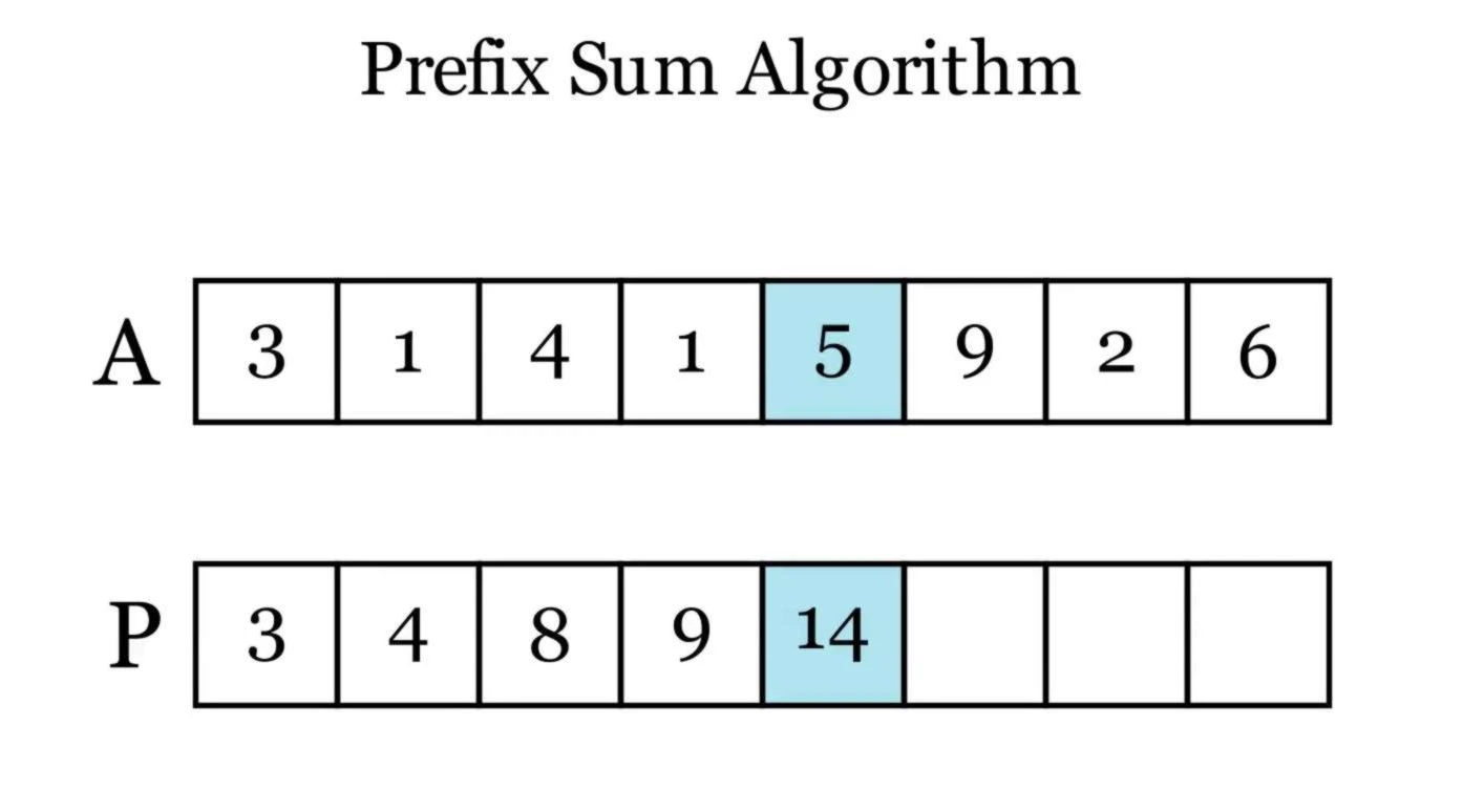 Figura 11.1.1.1.A - Step in the Prefix Sum Algorithm: The image shows the calculation of the fifth element of the prefix sum array $P$ from the original array $A$.
Compute $P$:
- $P[0] = A[0] = 3$
- $P[1] = P[0] + A[1] = 3 + 1 = 4$
- $P[2] = P[1] + A[2] = 4 + 4 = 8$
- $P[3] = P[2] + A[3] = 8 + 1 = 9$
- $P[4] = P[3] + A[4] = 9 + 5 = 14$
- $P[5] = P[4] + A[5] = 14 + 9 = 23$
- $P[6] = P[5] + A[6] = 23 + 2 = 25$
- $P[7] = P[6] + A[7] = 25 + 6 = 31$
Resulting prefix sum array:
\[P = [3, 4, 8, 9, 14, 23, 25, 31]\]Step 2: Perform Range Sum Queries
Example Query: Find the sum of elements from index $2$ to $5$ in $A$.
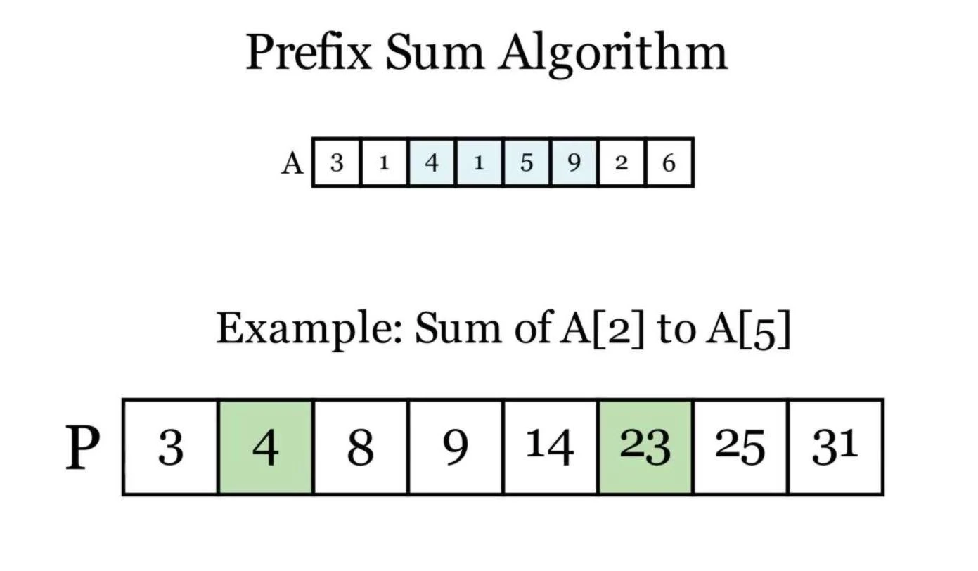 Figura 11.1.1.1.A - The image illustrates how the prefix sum array $P$ is constructed from the original array $A$. Example shows the sum calculation from $A[2]$ to $A[5]$ using the prefix sums.
- Compute: Since $i = 2 > 0$, use $\text{Sum}(2, 5) = P[5] - P[1]$
- Calculate: $\text{Sum}(2, 5) = 23 - 4 = 19$
- Verification:
- Sum of $A[2]$ to $A[5]$:
- $A[2] + A[3] + A[4] + A[5] = 4 + 1 + 5 + 9 = 19$
- Sum of $A[2]$ to $A[5]$:
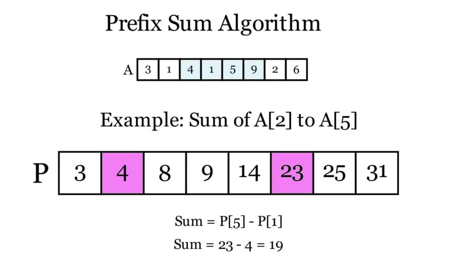 Figura 11.1.1.1.A - The image demonstrates how to use the prefix sum array $P$ to calculate the sum of elements from $A[2]$ to $A[5]$. The calculation is done using the formula $P[5] - P[1]$, resulting in $23 - 4 = 19$.
11.1.1.2. Complexity Analysis
The Prefix Sum Array algorithm’s complexity can be analyzed by considering its two main operations: constructing the prefix sum array and performing range sum queries.
In the construction phase, we initialize the prefix sum array $P$ by setting $P[0] = A[0]$, which requires constant time $O(1)$. Then, for each index $i$ from $1$ to $n - 1$, we compute $P[i] = P[i - 1] + A[i]$. This loop runs for $n - 1$ iterations, and each iteration involves a single addition operation, which is a constant-time operation $O(1)$. Therefore, the total time complexity for constructing the prefix sum array is:
\[O(1) + (n - 1) \times O(1) = O(n)\]Thus, the construction of the prefix sum array has a linear time complexity of $O(n)$. Regarding space complexity, we require an additional array $P$ of size $n$ to store the prefix sums, resulting in an extra space complexity of $O(n)$.
For performing a range sum query to calculate the sum of elements from index $i$ to $j$ in the original array $A$, we utilize the prefix sum array $P$. If $i = 0$, the sum is simply $P[j]$, which is retrieved in constant time $O(1)$. If $i > 0$, the sum is calculated as $P[j] - P[i - 1]$, involving two array accesses and one subtraction, all of which are constant-time operations. Therefore, each range sum query is executed in $O(1)$ time.
The space complexity for executing queries is $O(1)$, as no additional space is required beyond the already constructed prefix sum array.
In conclusion, the Prefix Sum Array algorithm has a time complexity of $O(n)$ for the preprocessing step of constructing the prefix sum array and $O(1)$ time per range sum query. The overall space complexity is $O(n)$ due to the storage of the prefix sum array. This efficiency makes the algorithm particularly useful when dealing with multiple range sum queries on a static array, as it significantly reduces the time complexity per query from $O(n)$ to $O(1)$ after the initial preprocessing.
11.1.1.3. Typical Problem: The Plate Balancer (Problem 2)
In a famous restaurant, Chef André is known for his incredible skill in balancing plates. He has a long table with several plates, each containing a different amount of food. André wants to find the “Magic Plate” - the plate where, when he places his finger underneath it, the weight of the food on the left and right balances perfectly.
Given a list of $plates$, where each number represents the weight of the food on each plate, your task is to help André find the index of the Magic Plate. The Magic Plate is the one where the sum of the weights of all plates to its left is equal to the sum of the weights of all plates to its right.
If André places his finger under the leftmost plate, consider the weight on the left as $0$. The same applies if he chooses the rightmost plate.
Return the leftmost Magic Plate index. If no such plate exists, return $-1$.
Example 1:
Input: $plates = [3,1,5,2,2]$
Output: $2$
Explanation:
The Magic Plate is at index $2$.
- Weight on the left = $plates[0] + plates[1] = 3 + 1 = 4$
- Weight on the right = $plates[3] + plates[4] = 2 + 2 = 4$
Example 2:
Input: $plates = [1,2,3]$
Output: $-1$
Explanation:
There is no plate that can be the Magic Plate.
Example 3:
Input: $plates = [2,1,-1]$
Output: $0$
Explanation:
The Magic Plate is the first plate.
- Weight on the left = $0$ (no plates to the left of the first plate)
- Weight on the right = $plates[1] + plates[2] = 1 + (-1) = 0$
Constraints:
\[1 \leq plates.length \leq 10^4\] \[-1000 \leq plates[i] \leq 1000\]Note: André is very skilled, so don’t worry about the real-world physics of balancing plates. Focus only on the mathematical calculations!
11.1.1.3.A Naïve Solution
This solution is considered naïve because it doesn’t take advantage of any precomputation or optimization techniques such as the Prefix Sum Array. Instead, it recalculates the sum of elements to the left and right of each plate using two separate loops for every plate. This leads to a time complexity of $O(n^2)$, as for each plate, the entire array is traversed twice — once for the left sum and once for the right sum.
A developer who writes this kind of code typically has a basic understanding of problem-solving but might not be familiar with more advanced algorithms or computational complexity analysis. They often rely on straightforward, brute-force approaches, focusing on getting a working solution without considering performance for large datasets. While this approach works for small inputs, it quickly becomes inefficient for larger ones due to its quadratic complexity.
The following is a Python pseudocode version of the naïve C++ solution, using the same variables and logic:
def find_magic_plate_naive(plates):
    n = len(plates)

    # Check every plate to see if it's the Magic Plate
    for i in range(n):
        left_sum = 0
        right_sum = 0

        # Calculate sum of elements to the left of plate i
        for j in range(i):
            left_sum += plates[j]

        # Calculate sum of elements to the right of plate i
        for j in range(i + 1, n):
            right_sum += plates[j]

        # If left and right sums are equal, return the current index
        if left_sum == right_sum:
            return i

    # If no Magic Plate found, return -1
    return -1

# Example usage
plates = [3, 1, 5, 2, 2]
result = find_magic_plate_naive(plates)
print(result)  # Should print 2
The following C++20 code implements a naïve solution to the problem of finding the Magic Plate. It uses a brute-force approach by iterating through each plate and calculating the sum of all plates to its left and right using two separate loops. While this method successfully solves the problem for small input sizes, it lacks efficiency, resulting in a time complexity of $O(n^2)$. This approach is typical of developers who prioritize a working solution over performance optimization, as it recalculates sums repeatedly without leveraging more advanced techniques such as the Prefix Sum Array.
#include <iostream>
#include <vector>

using namespace std;

// Function to find the index of the Magic Plate without optimization
int find_magic_plate_naive(const vector<int>& plates) {
    int n = plates.size();

    // Check every plate to see if it's the Magic Plate
    for (int i = 0; i < n; ++i) {
        int left_sum = 0;
        int right_sum = 0;

        // Calculate sum of elements to the left of plate i
        for (int j = 0; j < i; ++j) {
            left_sum += plates[j];
        }

        // Calculate sum of elements to the right of plate i
        for (int j = i + 1; j < n; ++j) {
            right_sum += plates[j];
        }

        // If left and right sums are equal, return the current index
        if (left_sum == right_sum) {
            return i;
        }
    }

    // If no Magic Plate found, return -1
    return -1;
}

int main() {
    // Example 1: plates = [3, 1, 5, 2, 2]
    vector<int> plates1 = { 3, 1, 5, 2, 2 };
    int result1 = find_magic_plate_naive(plates1);
    cout << "Magic Plate index for plates1: " << result1 << endl;

    // Example 2: plates = [1, 2, 3]
    vector<int> plates2 = { 1, 2, 3 };
    int result2 = find_magic_plate_naive(plates2);
    cout << "Magic Plate index for plates2: " << result2 << endl;

    // Example 3: plates = [2, 1, -1]
    vector<int> plates3 = { 2, 1, -1 };
    int result3 = find_magic_plate_naive(plates3);
    cout << "Magic Plate index for plates3: " << result3 << endl;

    return 0;
}
The C++20 code implements a solution to the Magic Plate problem by iterating over each plate and calculating the sum of the plates to its left and right. For each plate, two separate loops are used: one for calculating the left sum and another for calculating the right sum. The outer loop runs through all the plates, starting from the first plate to the last, and for each plate, the two sums are calculated to determine if it is the Magic Plate.
The left sum is calculated by iterating from the first plate up to, but not including, the current plate. As the code checks plates further down the list, the left sum loop becomes longer, meaning that plates near the end of the list require more iterations. Similarly, the right sum is calculated by looping through the plates to the right of the current plate. This right sum loop becomes longer for plates near the beginning of the list. The code compares these two sums, and if they are equal, the current plate index is returned as the solution. If no such plate is found, the function returns -1.
In terms of complexity, the time required to calculate the left and right sums for each plate depends on the position of the plate in the list. For the $i^{th}$ plate, the left sum takes approximately $O(i)$ iterations, while the right sum takes $O(n-i-1)$ iterations, where $n$ is the total number of plates. Since these calculations are done for every plate, the overall time complexity of the algorithm is $O(n^2)$. The space complexity is $O(1)$ because no additional arrays or data structures are created; the sums are calculated using simple scalar variables.
The following table summarizes the time and space complexities of each step in the algorithm:
| Step | Operation | Time Complexity | Space Complexity |
|---|---|---|---|
| Left Sum Calculation | Calculating sum of elements to the left of each plate | $O(i)$ | $O(1)$ |
| Right Sum Calculation | Calculating sum of elements to the right of each plate | $O(n-i-1)$ | $O(1)$ |
| Outer Loop (Plates Iteration) | Looping through each plate | $O(n)$ | $O(1)$ |
| Overall Complexity | Total time and space complexities | $O(n^2)$ | $O(1)$ |
This approach, while correct, leads to a quadratic time complexity of $O(n^2)$ because it recalculates the sums from scratch for every plate. The space complexity remains constant at $O(1)$, as no extra space is required beyond the scalar variables for sum calculation. Nevertheless, there are better solutions.
11.1.1.3.B Prefix Sum Array Solution
Let’s start solving the problem “The Plate Balancer” using the Prefix Sum Array algorithm, using Python to create a pseudocode:
def find_magic_plate(plates):
    n = length(plates)

    # Create prefix sum array
    prefix_sum = [0] * (n + 1)
    for i in range(1, n + 1):
        prefix_sum[i] = prefix_sum[i-1] + plates[i-1]

    # Calculate total sum
    total_sum = prefix_sum[n]

    # Find magic plate
    for i in range(1, n + 1):
        left_sum = prefix_sum[i-1]
        right_sum = total_sum - prefix_sum[i]

        if left_sum == right_sum:
            return i - 1  # Return 0-based index

    # If no magic plate found
    return -1

# Example usage
plates = [3, 1, 5, 2, 2]
result = find_magic_plate(plates)
print(result)  # Should print 2

plates = [1, 2, 3]
result = find_magic_plate(plates)
print(result)  # Should print -1

plates = [2, 1, -1]
result = find_magic_plate(plates)
print(result)  # Should print 0
Now a solution using C++ 20 to implement the Prefix Sum Array algorithm without any consideration about verbosity:
#include <iostream>
#include <vector>

using namespace std;

// Function to find the index of the Magic Plate
int find_magic_plate(const vector<int>& plates) {
    int n = plates.size();

    // If there is only one plate, it is automatically the Magic Plate
    if (n == 1) return 0;

    // Create a prefix sum array to store the cumulative sum up to each plate
    vector<int> prefix_sum(n + 1, 0);

    // Build the prefix sum array where each element contains the sum of elements up to that index
    for (int i = 1; i <= n; ++i) {
        prefix_sum[i] = prefix_sum[i - 1] + plates[i - 1];
    }

    // Calculate total sum (optional step, just for clarity)
    int total_sum = prefix_sum[n];

    // Check for each plate if the left sum equals the right sum
    for (int i = 1; i <= n; ++i) {
        // Left sum is the sum of elements before the current plate
        int left_sum = prefix_sum[i - 1];

        // Right sum is the total sum minus the current prefix sum
        int right_sum = total_sum - prefix_sum[i];

        // If the left and right sums are equal, return the current index (0-based)
        if (left_sum == right_sum) {
            return i - 1;
        }
    }

    // If no Magic Plate is found, return -1
    return -1;
}

int main() {
    // Example 1: plates = [3, 1, 5, 2, 2]
    vector<int> plates1 = { 3, 1, 5, 2, 2 };
    int result1 = find_magic_plate(plates1);
    cout << "Magic Plate index for plates1: " << result1 << endl;

    // Example 2: plates = [1, 2, 3]
    vector<int> plates2 = { 1, 2, 3 };
    int result2 = find_magic_plate(plates2);
    cout << "Magic Plate index for plates2: " << result2 << endl;

    // Example 3: plates = [2, 1, -1]
    vector<int> plates3 = { 2, 1, -1 };
    int result3 = find_magic_plate(plates3);
    cout << "Magic Plate index for plates3: " << result3 << endl;

    return 0;
}
The code implements the Prefix Sum Array algorithm to solve the problem The Plate Balancer. The approach starts by creating a prefix sum array (prefix_sum), which stores the cumulative sum of elements from the original plates array. The construction of this prefix sum array has a time complexity of $O(n)$, where $n$ is the number of plates. The Prefix Sum Array is built in such a way that for each index $i$, the value prefix_sum[i] contains the sum of all elements from plates[0] to plates[i-1]. This allows the sum of elements to the left of a given index to be computed in constant time $O(1)$ by simply accessing prefix_sum[i-1].
The construction of the Prefix Sum Array takes linear time $O(n)$ and requires additional space $O(n)$ for the array. For each plate, calculating the left and right sums is constant in time $O(1)$ due to the prefix sum array, but this is done $n$ times, resulting in $O(n)$ overall. The total sum is derived from the last value of the Prefix Sum Array, which is computed in constant time $O(1)$.
After building the Prefix Sum Array, the code uses it to calculate the left and right sums for each plate. The left sum of a plate at index $i$ is given by prefix_sum[i-1], while the right sum is derived by subtracting prefix_sum[i] from the total sum (total_sum). If the left and right sums are equal, the index of the plate is returned as the Magic Plate. Otherwise, the loop continues to check all plates. If no balanced plate is found, the code returns -1, indicating that there is no Magic Plate.
The implementation follows the Prefix Sum Array algorithm efficiently, constructing the array in linear time $O(n)$, and checking if a plate is the Magic Plate in constant time $O(1)$ for each plate. The logic in C++20 utilizes standard functions such as std::vector, ensuring simplicity and clarity in the code. The identifiers have been adjusted to match those from the Python pseudocode, maintaining the same logic and structure as the original algorithm. Below is a detailed analysis of the time and space complexities for each operation in the C++20 implementation:
| Step | Operation | Time Complexity | Space Complexity |
|---|---|---|---|
| Prefix Sum Array Construction | Building the prefix sum array prefix_sum |
$O(n)$ | $O(n)$ |
| Left and Right Sum Calculation | Calculating left and right sums for each plate | $O(1)$ per plate | $O(n)$ (reusing prefix sum) |
| Total Sum Calculation | Calculating the total sum using the prefix sum array | $O(1)$ | $O(n)$ |
| Loop Through Plates | Checking all plates for the Magic Plate | $O(n)$ | $O(1)$ |
| Overall Complexity | Total time and space complexities | $O(n)$ | $O(n)$ |
11.1.1.3.C Competitive Solution
The following C++20 code implements the Prefix Sum Array algorithm, with several optimizations designed to reduce typing effort in a competitive programming context. We eliminated the use of functions, as the entire code is kept within the main block, avoiding the overhead of function calls. This approach prioritizes minimal typing and fast execution by copying and pasting the logic rather than encapsulating it into reusable components.
Key changes made:
-
Use of
usingfor shorter variable names: We introducedusingdirectives to reduce the typing for commonly used variables. For instance,prefix_sumbecameps,total_sumbecamets, andplatesbecamepl. This allows us to minimize the amount of text written while keeping the code readable and maintainable in a fast-paced environment. We let comments in following code but not in the real competitive code available in github. -
Reuse of the same array for multiple test cases: Instead of declaring multiple arrays for different input examples, we reuse the same array
pland the variablenfor the array size. By resettingplandnfor each example, we save both memory and typing effort, while maintaining clarity. -
Hardcoded input examples: The input examples are directly written into the code (hardcoded), as is typical in competitive programming when no external input is required. The three provided examples are executed sequentially without the need for interactive input, allowing us to focus purely on solving the problem quickly.
-
Avoidance of function calls: We opted to avoid wrapping the Prefix Sum Array logic into functions to eliminate the slight cost of function calls. This decision was driven by the understanding that, in a competitive environment, even minimal overheads can accumulate and impact performance. Instead, we simply copied and pasted the algorithm, leveraging the simplicity and speed of direct logic execution.
Warnings:
During the development of this code, some warnings arose, such as a potential arithmetic overflow when performing summations and a warning about the conversion from size_t to int. To mitigate the risk of overflow, we made adjustments by using long long for the array and sums. However, the warning regarding the size_t to int conversion persists. This conversion warning arises because size_t is often used for the size of arrays, but we assign it to an int type. While this may lead to data loss in rare edge cases with very large data sizes, in the context of competitive programming where input sizes are usually constrained, this warning can be safely ignored.
Moreover, reducing the typing effort is crucial in competitive environments, and using int is often the most efficient approach when dealing with moderately sized inputs, which are common in contests. As such, we chose to keep this conversion despite the warning, knowing that it will not significantly affect the correctness of our solution for typical competition scenarios.
In C++20,
size_tis an unsigned integer type, typically used to represent the size of objects or memory blocks. It is an alias for an unsigned integer that can hold the size of the largest object your system can handle. Its size depends on the architecture of the system:
- On 32-bit systems,
size_tis typically 4 bytes (32 bits), which means it can hold values from 0 to $2^{32} - 1$.- On 64-bit systems,
size_tis typically 8 bytes (64 bits), which means it can hold values from 0 to $2^{64} - 1$.Typical Sizes of
int,long long, andsize_t: On most modern systems, the sizes of these types are as follows (though they can vary depending on the platform and architecture):
int: 4 bytes (32 bits): Range: $-2^{31}$ to $2^{31} - 1$long long: 8 bytes (64 bits): Range: $-2^{63}$ to $2^{63} - 1$ >size_t: 4 bytes (32 bits) on 32-bit systems, with a range from 0 to $2^{32} - 1$ and 8 bytes (64 bits) on 64-bit systems, with a range from 0 to $2^{64} - 1$.Since
size_tis unsigned, it can store only non-negative values, making it ideal for representing sizes and lengths where negative numbers don’t make sense (e.g., array indices, sizes of memory blocks).Difference Between
++iandi++
++iis the pre-increment operator, which increments the value ofifirst and then returns the incremented value.i++is the post-increment operator, which returns the current value ofifirst and then increments it.The main difference between the two is in performance when used in certain contexts, particularly with non-primitive types like iterators. Using
++iis slightly more efficient thani++becausei++might involve creating a temporary copy of the value before incrementing, while++imodifies the value directly. For example:int i = 0; int a = ++i; // a = 1, i = 1 (pre-increment: increment first, then use the value) int b = i++; // b = 1, i = 2 (post-increment: use the value first, then increment)
Below is the final competitive, and ugly, code:
#include <iostream>
#include <vector>

using namespace std;

using ps = vector<int>;  // Alias for prefix_sum as a vector of long long
using ts = int;          // Alias for total_sum as long long
using pl = vector<int>;  // Alias for plates as a vector of int
using vi = vector<int>;  // Alias for vector of int (similar to vi)

int main() {
    vi pl;
    int n;
    vi ps;

    pl = {3, 1, 5, 2, 2};
    n = pl.size();
    ps = vi(n + 1, 0);
    for (int i = 1; i <= n; ++i) ps[i] = ps[i - 1] + pl[i - 1];
    ts = ps[n];
    for (int i = 1; i <= n; ++i) {
        int ls = ps[i - 1], rs = ts - ps[i];
        if (ls == rs) {
            cout << i - 1 << endl;
            break;
        }
        if (i == n) cout << -1 << endl;
    }

    pl = {1, 2, 3};
    n = pl.size();
    ps = vi(n + 1, 0);
    for (int i = 1; i <= n; ++i) ps[i] = ps[i - 1] + pl[i - 1];
    ts = ps[n];
    for (int i = 1; i <= n; ++i) {
        int ls = ps[i - 1], rs = ts - ps[i];
        if (ls == rs) {
            cout << i - 1 << endl;
            break;
        }
        if (i == n) cout << -1 << endl;
    }

    pl = {2, 1, -1};
    n = pl.size();
    ps = vi(n + 1, 0);
    for (int i = 1; i <= n; ++i) ps[i] = ps[i - 1] + pl[i - 1];
    ts = ps[n];
    for (int i = 1; i <= n; ++i) {
        int ls = ps[i - 1], rs = ts - ps[i];
        if (ls == rs) {
            cout << i - 1 << endl;
            break;
        }
        if (i == n) cout << -1 << endl;
    }

    return 0;
}
11.1.2. Algorithm: Difference Array - Efficient Range Updates
The Difference Array algorithm is a powerful technique for handling multiple range update operations efficiently. It’s particularly useful when you need to perform many updates on an array and only query the final result after all updates are complete. Optimizes range updates to $O(1)$ by storing differences between adjacent elements.
The Difference Array algorithm shines in various scenarios where multiple range updates are required, and the final result needs to be computed only after all updates have been applied. Here are some common applications where this technique proves to be particularly effective:
- Range update queries: When you need to perform multiple range updates and only query the final array state.
- Traffic flow analysis: Modeling entry and exit points of vehicles on a road.
- Event scheduling: Managing overlapping time slots or resources.
- Image processing: Applying filters or adjustments to specific regions of an image.
- Time series data: Efficiently updating ranges in time series data.
- Competitive programming: Solving problems involving multiple range updates.
Consider an array $A$ of size $n$. The difference array $D$ is defined as:
\[D[i] = \begin{cases} A[i] - A[i-1], & \text{if } i > 0 \\ A[i], & \text{if } i = 0 \end{cases}\]Each element in $D$ represents the difference between consecutive elements in $A$. The key property of the difference array is that a range update on $A$ can be performed using only two operations on $D$.
To add a value $x$ to all elements in $A$ from index $l$ to $r$ (inclusive), we do:
\[D[l] += x\] \[D[r+1] -= x (\text{if} r+1 < n)\]After all updates, we can reconstruct $A$ from $D$ using:
\[A[i] = \sum_{j=0}^i D[j]\]This technique allows for $O(1)$ time complexity for each range update operation.
Let’s prove that the range update operation on $D$ correctly reflects the change in $A$.
-
For $i < l$:
\[A'[i] = \sum_{j=0}^i D'[j] = \sum_{j=0}^i D[j] = A[i]\] -
For $l \leq i \leq r$:
\[\begin{aligned} A'[i] &= \sum_{j=0}^i D'[j] \\ &= \sum_{j=0}^{l-1} D[j] + (D[l] + x) + \sum_{j=l+1}^i D[j] \\ &= (\sum_{j=0}^i D[j]) + x \\ &= A[i] + x \end{aligned}\] -
For $i > r$:
\[\begin{aligned} A'[i] &= \sum_{j=0}^i D'[j] \\ &= \sum_{j=0}^{l-1} D[j] + (D[l] + x) + \sum_{j=l+1}^r D[j] + (D[r+1] - x) + \sum_{j=r+2}^i D[j] \\ &= (\sum_{j=0}^i D[j]) + x - x \\ &= A[i] \end{aligned}\]
This proves that the range update operation on $D$ correctly reflects the desired change in $A$.
11.1.2.1 Difference Array Algorithm Explained in Plain English
-
Initialize the Difference Array
Given an original array $A$ of size $n$, we create a difference array $D$ as follows:
- For each index $i$ from $0$ to $n - 1$:
- If $i = 0$:
- Set $D[0] = A[0]$.
- Else:
- Set $D[i] = A[i] - A[i - 1]$.
This difference array $D$ represents the changes between consecutive elements in $A$.
-
Perform Range Updates
To add a value $x$ to all elements between indices $l$ and $r$ (inclusive) in $A$, we update $D$:
- Add $x$ to $D[l]$:
- Update $D[l] = D[l] + x$.
- If $r + 1 < n$:
- Subtract $x$ from $D[r + 1]$:
- Update $D[r + 1] = D[r + 1] - x$.
These two updates in $D$ ensure that when we reconstruct $A$, the value $x$ is added to all elements from $l$ to $r$.
-
Reconstruct the Updated Array
After all range updates, we can rebuild the updated array $A$:
- Set $A[0] = D[0]$.
- For each index $i$ from $1$ to $n - 1$:
- Set $A[i] = A[i - 1] + D[i]$.
This step accumulates the differences to get the final values in $A$.
Let’s walk through an example to see how the algorithm works.
Suppose we have the array:
\[A = [2, 3, 5, 7, 11]\]-
Initialize $D$
Compute $D$:
- $D[0] = A[0] = 2$
- $D[1] = A[1] - A[0] = 3 - 2 = 1$
- $D[2] = A[2] - A[1] = 5 - 3 = 2$
- $D[3] = A[3] - A[2] = 7 - 5 = 2$
- $D[4] = A[4] - A[3] = 11 - 7 = 4$
So,
\[D = [2, 1, 2, 2, 4]\] -
Perform a Range Update
We want to add $x = 3$ to all elements from index $l = 1$ to $r = 3$.
- Update $D[1]$:
- $D[1] = D[1] + 3 = 1 + 3 = 4$
- Since $r + 1 = 4 < n = 5$, update $D[4]$:
- $D[4] = D[4] - 3 = 4 - 3 = 1$
Updated $D$:
\[D = [2, 4, 2, 2, 1]\] -
Reconstruct the Updated Array
Rebuild $A$ using the updated $D$:
- $A[0] = D[0] = 2$
- $A[1] = A[0] + D[1] = 2 + 4 = 6$
- $A[2] = A[1] + D[2] = 6 + 2 = 8$
- $A[3] = A[2] + D[3] = 8 + 2 = 10$
- $A[4] = A[3] + D[4] = 10 + 1 = 11$
Final updated array:
\[A = [2, 6, 8, 10, 11]\] -
Verification
- The elements from index $1$ to $3$ have been increased by $3$.
- Original $A[1..3] = [3, 5, 7]$
- Updated $A[1..3] = [6, 8, 10]$
The Difference Array algorithm optimizes multiple range updates by reducing the time complexity to $O(1)$ per update. It is especially useful when dealing with scenarios that require numerous range modifications followed by queries for the final array state.
11.1.2.1.A Example Problem
Starting with $N(1 \leq N \leq 1,000,000, N \text{ odd})$ empty stacks. Beatriz receives a sequence of $K$ instructions $(1 \leq K \leq 25,000)$, each in the format “A B”, which means that Beatriz should add a new layer of hay to the top of each stack in the interval $A..B$. Calculate the median of the heights after the operations.
Input: $N = 7, K = 4$ Example Output:
3 5
5 5
2 4
4 6
Output:
1
Heights after updates: 0, 0, 1, 1, 2, 3, 3
Final height: 0 1 1 2 3 3 3
Indices: 1 2 3 4 5 6 7
def range_update(diff, l, r, x):
    diff[l] += x
    if r + 1 < len(diff):
        diff[r + 1] -= x

def reconstruct_heights(diff):
    heights = [0] * len(diff)
    heights[0] = diff[0]
    for i in range(1, len(diff)):
        heights[i] = heights[i-1] + diff[i]
    return heights

# Hardcoded inputs
N = 7  # Number of stacks
K = 4  # Number of instructions
instructions = [
    (3, 5),
    (5, 5),
    (2, 4),
    (4, 6)
]

# Initialize difference array
diff = [0] * (N + 1)

# Apply all instructions
for A, B in instructions:
    range_update(diff, A - 1, B - 1, 1)  # -1 for 0-based indexing

# Reconstruct final heights
final_heights = reconstruct_heights(diff)

# Print final heights for verification
print("Final heights:", final_heights[:-1])  # Exclude the last element as it's not part of the original array

# Calculate the median
sorted_heights = sorted(final_heights[:-1])
if N % 2 == 1:
    median = sorted_heights[N // 2]
else:
    median = (sorted_heights[(N - 1) // 2] + sorted_heights[N // 2]) // 2

print("Median height:", median)*Output**: [2, 5, 3, 0]
Algorithm Implementation in C++20:
#include <iostream>
#include <vector>
#include <algorithm>
#include <numeric>

using namespace std;

// Function to perform range update on the difference array
void range_update(vector<int>& diff, int l, int r, int x) {
    diff[l] += x;
    if (r + 1 < static_cast<int>(diff.size())) {
        diff[r + 1] -= x;
    }
}

// Function to reconstruct the final heights from the difference array
vector<int> reconstruct_heights(const vector<int>& diff) {
    vector<int> heights(diff.size());
    partial_sum(diff.begin(), diff.end(), heights.begin());
    return heights;
}

int main() {
    // Hardcoded inputs based on the example in the image
    int N = 7;  // Number of stacks
    int K = 4;  // Number of instructions
    vector<pair<int, int>> instructions = {
        {3, 5},
        {5, 5},
        {2, 4},
        {4, 6}
    };

    vector<int> diff(N + 1, 0);  // Difference array initialized with 0s

    // Apply all instructions
    for (const auto& [A, B] : instructions) {
        range_update(diff, A - 1, B - 1, 1);  // -1 for 0-based indexing
    }

    vector<int> final_heights = reconstruct_heights(diff);

    // Print final heights for verification
    cout << "Final heights: ";
    for (int height : final_heights) {
        cout << height << " ";
    }
    cout << endl;

    // Sort the heights to find the median
    sort(final_heights.begin(), final_heights.end());

    // Calculate the median
    int median;
    if (N % 2 == 1) {
        median = final_heights[N / 2];
    } else {
        median = (final_heights[(N - 1) / 2] + final_heights[N / 2]) / 2;
    }

    cout << "Median height: " << median << endl;

    return 0;
}
11.1.2.2 Complexity Analysis
The Difference Array algorithm offers significant performance benefits, particularly for scenarios involving multiple range updates. Let’s examine its complexity:
-
Range Update Operation: The beauty of this algorithm lies in its constant-time range updates. Regardless of the size of the range being updated, we only modify two elements in the difference array $D$. This results in a time complexity of $O(1)$ for each range update operation.
-
Array Reconstruction: When we need to reconstruct the original array $A$ from the difference array $D$, we perform a single pass through $D$, computing cumulative sums. This operation has a time complexity of $O(n)$, where $n$ is the size of the array.
-
Space Complexity: The algorithm requires an additional array $D$ of the same size as the original array $A$. Therefore, the space complexity is $O(n)$.
The efficiency of this algorithm becomes apparent when dealing with multiple range updates followed by a single query or reconstruction. In such scenarios, we can perform $m$ range updates in $O(m)$ time, followed by a single $O(n)$ reconstruction, resulting in a total time complexity of $O(m + n)$. This is significantly more efficient than performing $m$ range updates directly on the original array, which would take $O(mn)$ time.
| Operation | Time Complexity | Space Complexity |
|---|---|---|
| Initialization | $O(n)$ | $O(n)$ |
| Range update | $O(1)$ | $O(n)$ |
| Array reconstruction | $O(n)$ | $O(n)$ |
| Overall Complexity | $O(n + q)$ | $O(n)$ |
11.1.2.3. Typical Problem: Humidity Levels in a Greenhouse (Problem 1)
This problem is the same as the one described in section 11.1.1.3. To solve it, we need to efficiently compute the sum of even humidity readings after each adjustment without recalculating the entire sum each time. We start by calculating the initial sum $S$ of all even numbers in the $humidity$ array. For each adjustment $[\text{adjustment}, \, \text{sensor_index}]$, we first retrieve the original value $v = humidity[\text{sensor_index}]$. If $v$ is even, we subtract it from $S$ because its value will change and it may no longer be even. We then update the humidity reading to $v_{\text{new}} = v + \text{adjustment}$. If $v_{\text{new}}$ is even, we add it to $S$. This way, after each adjustment, $S$ accurately reflects the sum of even humidity readings. By updating $S$ incrementally, we avoid the need to sum over the entire array after each adjustment, thus optimizing the computation.
11.1.2.3.A. Naïve Solution
Algorithm:
-
Initialize an empty list called
resultsto store the sums of even values after each adjustment. -
For each adjustment $[adjustment, sensorIndex]$ in the
adjustmentslist:a. Update the corresponding sensor’s value in the
humidityarray: $humidity[sensorIndex] = humidity[sensorIndex] + adjustment$b. Calculate the sum of even values in the
humidityarray:- Initialize a variable
even_sumto 0 - For each value $h$ in
humidity:- If $h$ is even (i.e., $h \bmod 2 = 0$), add $h$ to
even_sum
- If $h$ is even (i.e., $h \bmod 2 = 0$), add $h$ to
c. Append
even_sumto theresultslist - Initialize a variable
-
Return the
resultslist
Implementation - Pseudo code:
def calculate_even_sum_after_adjustments(humidity, adjustments):
    # Inicializa uma lista para armazenar os resultados
    results = []

    # Para cada ajuste na lista de ajustes
    for adjustment, sensor_index in adjustments:
        # Atualiza o valor do sensor correspondente no array de umidade
        humidity[sensor_index] += adjustment

        # Calcula a soma dos valores pares na lista de umidade
        even_sum = 0
        for h in humidity:
            if h % 2 == 0:  # Verifica se o valor é par
                even_sum += h

        # Adiciona a soma atual dos valores pares na lista de resultados
        results.append(even_sum)

    # Retorna a lista de resultados
    return results

# Exemplo de uso:
humidity = [45, 52, 33, 64]
adjustments = [[5, 0], [-20, 1], [-14, 0], [18, 3]]
result = calculate_even_sum_after_adjustments(humidity, adjustments)
print(result)  # Saída: [166, 146, 132, 150]
Implementation - C++ 20:
#include <iostream>  // Includes the library for input and output operations.
#include <vector>    // Includes the library to use vectors.
#include <numeric>   // Includes the library that provides the accumulate function.

using namespace std;

// Function that adjusts the humidity levels and calculates the sum of even values after each adjustment.
vector<long long> adjustHumidity(vector<int>& humidity, const vector<vector<int>>& adjustments) {
    // Creates a vector to store the results, reserving enough space to avoid unnecessary reallocations.
    vector<long long> result;
    result.reserve(adjustments.size());

    // Iterates over each adjustment provided.
    for (const auto& adjustment : adjustments) {
        int value = adjustment[0];  // Extracts the adjustment value.
        int index = adjustment[1];  // Extracts the sensor index to be adjusted.

        // Updates the value in humidity[index] with the adjustment.
        humidity[index] += value;

        // Calculates the sum of even values in the humidity array after the update.
        long long sum = accumulate(humidity.begin(), humidity.end(), 0LL,
            [](long long acc, int val) {
                return acc + (val % 2 == 0 ? val : 0);  // Adds to the sum if the value is even.
            });

        // Adds the current sum of even values to the result vector.
        result.push_back(sum);
    }
    // Returns the vector containing the sum of even values after each adjustment.
    return result;
}

// Helper function to print the results in a formatted way.
void printResult(const vector<int>& humidity, const vector<vector<int>>& adjustments, const vector<long long>& result) {
    // Prints the initial humidity and the adjustments.
    cout << "**Input**: humidity = [";
    for (size_t i = 0; i < humidity.size(); ++i) {
        cout << humidity[i] << (i < humidity.size() - 1 ? ", " : "");  // Prints each humidity value, separating them with commas.
    }
    cout << "], adjustments = [";
    for (size_t i = 0; i < adjustments.size(); ++i) {
        // Prints each adjustment in the form [value, index].
        cout << "[" << adjustments[i][0] << "," << adjustments[i][1] << "]" << (i < adjustments.size() - 1 ? ", " : "");
    }
    cout << "]\n";

    // Prints the result after each adjustment.
    cout << "**Output**: ";
    for (long long res : result) {
        cout << res << " ";  // Prints each result, separating them by spaces.
    }
    cout << "\n\n";
}

int main() {
    // Example 1
    vector<int> humidity1 = { 45, 52, 33, 64 };  // Initial humidity vector.
    vector<vector<int>> adjustments1 = { {5,0}, {-20,1}, {-14,0}, {18,3} };  // Adjustment vector.
    cout << "Example 1:\n";
    auto result1 = adjustHumidity(humidity1, adjustments1);  // Calculates the results.
    printResult(humidity1, adjustments1, result1);  // Prints the results.

    // Example 2
    vector<int> humidity2 = { 40 };  // Initial humidity vector.
    vector<vector<int>> adjustments2 = { {12,0} };  // Adjustment vector.
    cout << "Example 2:\n";
    auto result2 = adjustHumidity(humidity2, adjustments2);  // Calculates the results.
    printResult(humidity2, adjustments2, result2);  // Prints the results.

    return 0;  // Indicates that the program terminated successfully.
}
The only noteworthy fragment in previous C++ implementation is the lambda function used to calculate the sum in:
// Calculates the sum of even values in the humidity array after the update.
        long long sum = accumulate(humidity.begin(), humidity.end(), 0LL,
            [](long long acc, int val) {
                return acc + (val % 2 == 0 ? val : 0);  // Adds to the sum if the value is even.
            });
This line calculates the sum of even values in the humidity array after the update. The accumulate function is used to iterate over the humidity array and sum only the even values. The first two parameters, humidity.begin() and humidity.end(), define the range of elements in the array to be processed. The third parameter, 0LL, initializes the accumulator with a value of $0$, where LL specifies that it is a long long integer.
The fourth parameter is a lambda function that takes two arguments: acc, which is the accumulated sum so far, and val, the current value being processed from the array. Inside the lambda function, the expression val % 2 == 0 ? val : 0 checks whether the current value val is even (i.e., divisible by 2). If val is even, it is added to the accumulator acc; otherwise, 0 is added, which does not affect the sum.
Thus, the final result of the accumulate function is the sum of only the even values in the array, which is then stored in the variable sum. Well, something needs a little bit of attention.
The
<numeric>library in C++ provides a collection of functions primarily focused on numerical operations. These functions are designed to simplify common tasks such as accumulating sums, performing inner products, calculating partial sums, and more. One of the most commonly used functions in this library isaccumulate, which is used to compute the sum (or other types of accumulation) of a range of elements in a container.The general syntax for the
accumulatefunction is:T accumulate(InputIterator first, InputIterator last, T init); T accumulate(InputIterator first, InputIterator last, T init, BinaryOperation op);
- InputIterator first, last: These define the range of elements to be accumulated. The
firstpoints to the beginning of the range, andlastpoints to one past the end of the range.- T init: This is the initial value of the accumulator, where the result of the accumulation will start.
- BinaryOperation op (optional): This is an optional custom function (usually a lambda or function object) that specifies how two elements are combined during the accumulation. If not provided, the function defaults to using the addition operator (
+).Example 1: Simple Accumulation (Summing Elements): In its simplest form,
accumulatecan be used to sum all elements in a range.#include <numeric> #include <vector> #include <iostream> int main() { std::vector<int> vec = {1, 2, 3, 4, 5}; int sum = std::accumulate(vec.begin(), vec.end(), 0); // Sum of all elements std::cout << sum; // Outputs: 15 return 0; }In this example,
accumulateis used with the addition operator (default behavior) to sum the elements in the vector.Example 2: Custom Accumulation Using a Lambda Function: A custom operation can be applied during accumulation by providing a binary operation. For instance, to multiply all elements instead of summing them:
int product = std::accumulate(vec.begin(), vec.end(), 1, [](int acc, int x) {
    return acc * x;
});
std::cout << product;  // Outputs: 120
Here, instead of summing, the lambda function multiplies the elements.
Key Features of
accumulate:
- Default behavior: When no custom operation is provided,
accumulatesimply adds the elements of the range, starting with the initial value.- Custom operations: By passing a custom binary operation,
accumulatecan perform more complex operations like multiplication, finding the maximum, or applying transformations.- Initial value: The initial value is critical for defining the result type and the starting point of the accumulation. For instance, starting the accumulation with
0results in a sum, while starting with1can be useful for calculating products.Example 3: Accumulating with Different Types
accumulatecan also work with different types by adjusting the initial value and operation. For example, accumulating floating-point values from integers:double avg = std::accumulate(vec.begin(), vec.end(), 0.0) / vec.size(); std::cout << avg; // Outputs: 3.0In this case, starting the accumulation with a double (
0.0) ensures that the result is a floating-point number.Limitations and Considerations:
- No built-in parallelism: The standard
accumulatefunction does not support parallel execution, meaning it processes elements sequentially. For parallel processing, alternative solutions like algorithms from the<execution>library introduced in C++17 are required.- Performance: The time complexity of
accumulateis $O(n)$, as it iterates over each element exactly once, applying the operation specified.Example 4: Custom Accumulation to Filter Elements You can use
accumulatein combination with a lambda to perform conditional accumulation. For example, to sum only even numbers:int even_sum = std::accumulate(vec.begin(), vec.end(), 0, [](int acc, int x) { return (x % 2 == 0) ? acc + x : acc; }); std::cout << even_sum; // Outputs: 6 (2 + 4)In this example, only the even numbers are added to the sum by applying a condition within the lambda function.
Finally, we need to clarify lambda functions in C++ 20.
Lambda functions in C++, available since C++ 11, are anonymous functions, meaning they do not have a name like regular functions. These are used when a function is needed only temporarily, typically for short operations, such as inline calculations or callback functions. Lambda functions are defined in place where they are used and can capture variables from their surrounding scope. Lambdas in C++ have been available since C++11, but in C++20, their capabilities were further expanded, making them more powerful and flexible.
The general syntax for a lambda function in C++ is as follows:
[capture](parameters) -> return_type {
    // function body
};
- Capture: Specifies which variables from the surrounding scope can be used inside the lambda. Variables can be captured by value
[=]or by reference[&]. You can also specify individual variables, such as[x]or[&x], to capture them by value or reference, respectively.- Parameters: The input parameters for the lambda function, similar to function arguments.
- Return Type: Optional in most cases, as C++ can infer the return type automatically. However, if the return type is ambiguous or complex, it can be specified explicitly using
-> return_type.- Body: The actual code to be executed when the lambda is called.
C++20 brought some new features to lambda functions. One of the most important improvements is the ability to use lambdas in immediate functions (with
consteval), and lambdas can now be default-constructed without capturing any variables. Additionally, lambdas in C++20 can use template parameters, allowing them to be more flexible and generic.Example 1: Basic Lambda Function: A simple example of a lambda function that sums two numbers:
auto sum = [](int a, int b) -> int {
    return a + b;
};
std::cout << sum(5, 3);  // Outputs: 8
Example 2: Lambda with Capture: In this example, a variable from the surrounding scope is captured by value:
int x = 10;
auto multiply = [x](int a) {
    return x * a;
};
std::cout << multiply(5);  // Outputs: 50
Here, the lambda captures
xby value and uses it in its body.Example 3: Lambda with Capture by Reference: In this case, the variable
yis captured by reference, allowing the lambda to modify it:int y = 20; auto increment = [&y]() { y++; }; increment(); std::cout << y; // Outputs: 21Example 4: Generic Lambda Function with C++20: With C++20, lambdas can now use template parameters, making them more generic:
auto generic_lambda = []<typename T>(T a, T b) {
    return a + b;
};
std::cout << generic_lambda(5, 3);      // Outputs: 8
std::cout << generic_lambda(2.5, 1.5);  // Outputs: 4.0
This lambda can add both integers and floating-point numbers by utilizing template parameters.
Key Improvements in C++20:
Default-constructed lambdas: In C++20, lambdas that do not capture any variables can now be default-constructed. This means they can be created and assigned to a variable without being immediately invoked or fully defined. This allows storing and passing lambdas for later use when default behavior is required.
auto default_lambda = [] {};  // Define a lambda with no capture or parameters
default_lambda();             // Call the lambda; valid as of C++20
This feature enables the initialization of lambdas for deferred execution.
Immediate lambdas: C++20 introduces consteval, which ensures that functions marked with this keyword are evaluated at compile-time. When used with lambdas, this feature guarantees that the lambda’s execution happens during compilation, and the result is already known by the time the program runs. A lambda used within a
constevalfunction enforces compile-time evaluation.In programming competitions,
constevallambdas are unlikely to be useful because contests focus on runtime performance, and compile-time evaluation does not offer any competitive advantage. Problems in contests rarely benefit from compile-time execution, as the goal is typically to optimize runtime efficiency.Consteval ensures that the function cannot be executed at runtime. If a function marked
constevalis invoked in a context that does not allow compile-time evaluation, it results in a compile-time error.Example:
consteval auto square(int x) {
    return [] (int y) { return y * y; }(x);
}
int value = square(5);  // Computed at compile-time
In this example, the lambda inside the
squarefunction is evaluated at compile-time, producing the result before the program starts execution.Since programming contests focus on runtime behavior and dynamic inputs, features like
constevalare not typically useful. Compile-time operations are not usually required in contests, where inputs are provided after the program has already started executing.Template lambdas: C++20 allows lambdas to accept template parameters, enabling generic behavior. This feature lets lambdas handle different data types without the need for function overloads or separate template functions. The template parameter is declared directly in the lambda’s definition, allowing the same lambda to adapt to various types.
Example:
auto generic_lambda = []<typename T>(T a, T b) {
    return a + b;
};
std::cout << generic_lambda(5, 3);      // Outputs: 8
std::cout << generic_lambda(2.5, 1.5);  // Outputs: 4.0
In this case, the lambda can process both integer and floating-point numbers, dynamically adapting to the types of its arguments.
Data Type Analysis in the adjustHumidity Function:
The choice of long long for the return type of the adjustHumidity function and for storing intermediate sums is made to ensure safety and prevent overflow in extreme cases:
- Array size: The problem specifies that there can be up to $10^4$ elements in the humidity array.
- Maximum element value: Each element in the array can have a value of up to $10^4$.
- Worst-case scenario: If all elements in the array are even and have the maximum value, the sum would be $10^4 \times 10^4 = 10^8$.
intlimit: In most implementations, aninthas 32 bits, with a maximum value of $2^{31} - 1 ≈ 2.15 \times 10^9$.- Safety margin: Although $10^8$ fits within an
int, it is best practice to leave a safety margin, especially considering there may be multiple adjustments that could further increase the values. long longguarantee: Along longis guaranteed to be at least 64 bits, providing a much larger range (up to $2^{63} - 1$ forsigned long long), which is more than sufficient for this problem.
By using long long, we ensure that no overflow occurs, even in extreme or unexpected cases. However, this could potentially lead to higher memory usage, which may exceed the limits in some competitive programming environments, depending on memory constraints.
Time and Space Complexity Analysis:
The current implementation recalculates the sum of even numbers in the humidity array after each adjustment using the std::accumulate function. This results in a time complexity of $O(n \times m)$, where $n$ is the size of the humidity array and $m$ is the number of adjustments in the adjustments list.
- Accumulation per adjustment: For each adjustment, the
std::accumulatefunction iterates over allnelements in thehumidityarray. This operation takes $O(n)$ time. - Total complexity: Since there are $m$ adjustments, the overall time complexity becomes $O(n \times m)$. This approach is inefficient for large values of $n$ and $m$ (e.g., if both $n$ and $m$ approach $10^4$), leading to performance issues in cases where the number of elements or adjustments is large.
The space complexity is primarily influenced by the size of the input arrays: The humidity array contains $n$ elements, each of which is an int, so the space required for this array is $O(n)$; The adjustments array contains $m$ adjustments, where each adjustment is a pair of integers. Therefore, the space required for this array is $O(m)$. Finally, the result vector stores $m$ results, each of type long long, so the space required for this vector is $O(m)$. In total, the space complexity is $O(n + m)$.
The usage of long long ensures that the results and intermediate sums are safe from overflow, but it may slightly increase memory usage compared to using int. The overall space requirements are manageable within typical constraints in competitive programming environments, where both $n$ and $m$ are capped at $10^4$.
11.1.2.3.B. Algorithm for a Slightly Less Naive Code
Let’s try a slightly less naive solution starting from we saw earlier: Initialize the variable even_sum with the value $0$ and create an empty list results to store the sums of even values after each adjustment.
Initially, calculate the sum of the even values in the humidity array. For each value $h$ in humidity, if $h$ is even (i.e., $h \bmod 2 = 0$), add $h$ to even_sum.
For each adjustment $[adjustment_value, sensor_index]$ in the adjustments list, check if the current value in humidity[sensor\_index] is even. If it is, subtract it from even_sum. Then, update the sensor’s value by adding adjustment\_value to the existing value:
Check if the new value in humidity[sensor\_index] is even. If it is, add it to even_sum. Add the current value of even_sum to the results list. Finally, return the results list.
Implementation - C++ 20:
#include <iostream>
#include <vector>

using namespace std;

// Function that adjusts humidity levels and calculates the sum of even values after each adjustment.
vector<long long> adjustHumidity(vector<int>& humidity, const vector<vector<int>>& adjustments) {
    // Initialize the sum of even numbers to zero.
    long long sum = 0;

    // Calculate the initial sum of even values in the humidity array.
    for (int h : humidity) {
        if (h % 2 == 0) {  // Check if the value is even.
            sum += h;  // Add to the sum if it's even.
        }
    }

    // Create a vector to store the results, reserving enough space to avoid unnecessary reallocations.
    vector<long long> result;
    result.reserve(adjustments.size());

    // Iterate through each adjustment provided.
    for (const auto& adjustment : adjustments) {
        int value = adjustment[0];  // Extract the adjustment value.
        int index = adjustment[1];  // Extract the index of the sensor to be adjusted.

        // Check if the current value in humidity[index] is even.
        if (humidity[index] % 2 == 0) {
            sum -= humidity[index];  // If it's even, subtract it from the sum of even numbers.
        }

        // Update the value in humidity[index] with the adjustment.
        humidity[index] += value;

        // Check if the new value in humidity[index] is even after the update.
        if (humidity[index] % 2 == 0) {
            sum += humidity[index];  // If it's even, add it to the sum of even numbers.
        }

        // Add the current sum of even values to the result vector.
        result.push_back(sum);
    }

    // Return the vector containing the sum of even values after each adjustment.
    return result;
}

// Helper function to print the results in a formatted way.
void printResult(const vector<int>& humidity, const vector<vector<int>>& adjustments, const vector<long long>& result) {
    // Print the initial humidity values and the adjustments.
    cout << "**Input**: humidity = [";
    for (size_t i = 0; i < humidity.size(); ++i) {
        cout << humidity[i] << (i < humidity.size() - 1 ? ", " : "");
    }
    cout << "], adjustments = [";
    for (size_t i = 0; i < adjustments.size(); ++i) {
        cout << "[" << adjustments[i][0] << "," << adjustments[i][1] << "]" << (i < adjustments.size() - 1 ? ", " : "");
    }
    cout << "]\n";

    // Print the result after each adjustment.
    cout << "**Output**: ";
    for (long long res : result) {
        cout << res << " ";
    }
    cout << "\n\n";
}

int main() {
    // Example 1
    vector<int> humidity1 = { 45, 52, 33, 64 };  // Initial humidity array.
    vector<vector<int>> adjustments1 = { {5,0}, {-20,1}, {-14,0}, {18,3} };  // Adjustment array.
    cout << "Example 1:\n";
    auto result1 = adjustHumidity(humidity1, adjustments1);  // Compute the results.
    printResult(humidity1, adjustments1, result1);  // Print the results.

    // Example 2
    vector<int> humidity2 = { 40 };  // Initial humidity array.
    vector<vector<int>> adjustments2 = { {12,0} };  // Adjustment array.
    cout << "Example 2:\n";
    auto result2 = adjustHumidity(humidity2, adjustments2);  // Compute the results.
    printResult(humidity2, adjustments2, result2);  // Print the results.

    return 0;  // Indicate that the program completed successfully.
}
This code adjusts the humidity levels in an array and computes the sum of even numbers after each adjustment. It begins by initializing the sum of even numbers from the humidity array, adding each even element to a running total. This sum is stored in the variable sum, which is later updated based on adjustments made to the humidity array.
For each adjustment in the adjustments list, the code checks if the value at the target sensor index (i.e., humidity[index]) is even. If it is, that value is subtracted from the running total. After updating the sensor’s value, the code checks again if the new value is even and adds it to the total if true. This ensures that only even numbers are considered in the running total, which is then stored in a results vector after each adjustment.
Finally, the results vector is returned, which contains the sum of even numbers in the humidity array after each adjustment. The printResult function is used to display the initial humidity values, the adjustments applied, and the resulting sums in a formatted manner.
The
autokeyword in C++ is used to automatically deduce the type of a variable at compile-time. This feature has been available since C++11, but with C++20, its functionality has been improved, allowing for greater flexibility in template functions, lambdas, and other contexts where type inference can simplify code. Theautokeyword is particularly useful when dealing with complex types, such as iterators, lambdas, or template instantiations, as it reduces the need for explicitly specifying types.When declaring a variable with
auto, the type is inferred from the initializer. This eliminates the need to explicitly specify the type, which can be especially useful when working with types that are long or difficult to express.auto x = 10; // x is automatically deduced as an int auto y = 3.14; // y is deduced as a double auto str = "Hello"; // str is deduced as a const char*In each case, the type of the variable is inferred based on the assigned value. This helps make code more concise and easier to maintain.
autoand Functions:In C++20, the
autokeyword can be used in function return types and parameters. The compiler deduces the return type or parameter type, allowing for greater flexibility in function definitions, especially with lambdas and template functions.Example:
auto add(auto a, auto b) {
   return a + b;
}

int main() {
   std::cout << add(5, 3);       // Outputs: 8
   std::cout << add(2.5, 1.5);   // Outputs: 4.0
}
In this example, the
addfunction can handle both integer and floating-point numbers because the types are deduced automatically. This simplifies function declarations, especially in template-like contexts.
autowith Lambdas and Template Functions:C++20 allows for more complex use cases of
autowithin lambdas and template functions. For instance, lambda expressions can useautoto deduce parameter types without explicitly specifying them. Additionally, theautokeyword can be combined with template parameters to create generic, flexible code.Example:
auto lambda = [](auto a, auto b) {
    return a + b;
};

std::cout << lambda(5, 3);        // Outputs: 8
std::cout << lambda(2.5, 1.5);    // Outputs: 4.0
Here, the lambda function uses
autoto deduce the types of its parameters, making it applicable to both integers and floating-point numbers.
A Parallel Competitive Code
Using parallel code in this problem offers a advantage by allowing the calculation of the sum of even humidity values to be distributed across multiple processing threads. This can improve performance, especially for large humidity arrays, as the reduce function could leverage parallel execution policies to sum even values concurrently, reducing overall runtime. However, in the current implementation, the sequential execution policy (exec_seq) is used to maintain order. Additionally, the Code 3 already employs techniques to reduce verbosity, such as type aliases (vi, vvi, vll) and the use of auto for type deduction, making the code cleaner and easier to maintain without sacrificing readability.
In ICPC programming competitions, extremely large input arrays are not typically common, as problems are designed to be solvable within strict time limits, often with manageable input sizes. However, in other competitive programming environments, such as online coding platforms or specific algorithm challenges, larger datasets may appear, requiring more optimized solutions. These scenarios may involve parallel processing techniques or more efficient algorithms to handle the increased computational load. While this problem’s input size is moderate, the techniques used here, like reducing verbosity with type aliases and utilizing reduce, ensure that the code can scale if needed.
Code 3 is already optimized to minimize function overhead, which can be an important factor in competitive programming. For instance, the entire algorithm is placed inside the main function, reducing the need for additional function calls and thus improving performance in time-sensitive environments.
Code 3:
#include <iostream>
#include <vector>
#include <numeric>
#include <execution>  // Necessary for execution policies in reduce

using namespace std;

// Aliases to reduce typing of long types
using vi = vector<int>;           // Alias for vector<int>
using vvi = vector<vector<int>>;  // Alias for vector of vectors of int
using vll = vector<long long>;    // Alias for vector<long long>
using exec_seq = execution::sequenced_policy; // Alias for execution::seq (sequential execution)

// Helper function to print the results in a formatted way.
void printResult(const vi& humidity, const vvi& adjustments, const vll& result) {
    // Prints the initial humidity array and the adjustments array.
    cout << "**Input**: humidity = [";
    for (size_t i = 0; i < humidity.size(); ++i) {
        // Print each humidity value, separating them with commas.
        cout << humidity[i] << (i < humidity.size() - 1 ? ", " : "");
    }
    cout << "], adjustments = [";
    for (size_t i = 0; i < adjustments.size(); ++i) {
        // Print each adjustment as [value, index], separating them with commas.
        cout << "[" << adjustments[i][0] << "," << adjustments[i][1] << "]" << (i < adjustments.size() - 1 ? ", " : "");
    }
    cout << "]\n";

    // Prints the results after each adjustment.
    cout << "**Output**: ";
    for (auto res : result) {  // Using `auto` to automatically deduce the type (long long)
        cout << res << " ";    // Print each result followed by a space.
    }
    cout << "\n\n";
}

int main() {
    // Example 1: Initialize the humidity vector and the adjustments to be made.
    vi humidity1 = { 45, 52, 33, 64 };  // Initial humidity levels for each sensor.
    vvi adjustments1 = { {5,0}, {-20,1}, {-14,0}, {18,3} };  // Adjustments in format {adjustment value, sensor index}.

    // Create a vector to store the results, reserving space to avoid reallocation during execution.
    vll result1;
    result1.reserve(adjustments1.size());

    // Process each adjustment for the humidity array.
    for (const auto& adjustment : adjustments1) {
        int value = adjustment[0];  // Get the adjustment value.
        int index = adjustment[1];  // Get the index of the sensor to be adjusted.

        // Apply the adjustment to the corresponding humidity value.
        humidity1[index] += value;

        // Calculate the sum of even values in the humidity array using the `reduce` function.
        auto sum = reduce(
            exec_seq{},              // Use sequential execution policy to maintain order.
            humidity1.begin(),       // Start iterator of the humidity vector.
            humidity1.end(),         // End iterator of the humidity vector.
            0LL,                     // Initial sum is 0 (as long long to avoid overflow).
            [](auto acc, auto val) { // Lambda function to accumulate even numbers.
                return acc + (val % 2 == 0 ? val : 0);  // Add to the sum only if the value is even.
            }
        );

        // Store the current sum of even values after the adjustment in the result vector.
        result1.push_back(sum);
    }

    // Print the results for the first example.
    cout << "Example 1:\n";
    printResult(humidity1, adjustments1, result1);

    // Example 2: Initialize the second humidity vector and the adjustments.
    vi humidity2 = { 40 };  // Initial humidity levels for the second example.
    vvi adjustments2 = { {12,0} };  // Adjustments for the second example.

    // Create a vector to store the results.
    vll result2;
    result2.reserve(adjustments2.size());

    // Process each adjustment for the second humidity array.
    for (const auto& adjustment : adjustments2) {
        int value = adjustment[0];  // Get the adjustment value.
        int index = adjustment[1];  // Get the index of the sensor to be adjusted.

        // Apply the adjustment to the corresponding humidity value.
        humidity2[index] += value;

        // Calculate the sum of even values in the humidity array using `reduce`.
        auto sum = reduce(
            exec_seq{},              // Use sequential execution policy to maintain order.
            humidity2.begin(),       // Start iterator of the humidity vector.
            humidity2.end(),         // End iterator of the humidity vector.
            0LL,                     // Initial sum is 0 (as long long to avoid overflow).
            [](auto acc, auto val) { // Lambda function to accumulate even numbers.
                return acc + (val % 2 == 0 ? val : 0);  // Add to the sum only if the value is even.
            }
        );

        // Store the current sum of even values after the adjustment in the result vector.
        result2.push_back(sum);
    }

    // Print the results for the second example.
    cout << "Example 2:\n";
    printResult(humidity2, adjustments2, result2);

    return 0;  // Indicate that the program finished successfully.
}
The core of the algorithm in Code 3 focuses on adjusting humidity levels based on a series of adjustments and then calculating the sum of even humidity values after each adjustment. The main part responsible for solving the problem involves iterating over each adjustment and performing two key operations: updating the humidity values and calculating the sum of even numbers in the updated array. This is done by:
-
Adjusting the Humidity: For each adjustment (which consists of an adjustment value and an index), the corresponding humidity value is updated by adding the adjustment value. This modifies the sensor reading at the specified index in the
humidityvector.Example:
humidity[index] += value;This line updates the humidity value at the sensor located at
indexby adding the providedvalue. -
Calculating the Sum of Even Values: After each adjustment, the algorithm calculates the sum of the even values in the
humidityarray. This is done using thereducefunction with a lambda function that filters and sums only the even numbers. The key here is that the algorithm iterates over the entirehumidityarray and sums the values that are divisible by 2.Example:
auto sum = reduce(
    exec_seq{},              // Sequential execution
    humidity.begin(),        // Start of the humidity array
    humidity.end(),          // End of the humidity array
    0LL,                     // Initial sum set to 0 (long long)
    [](auto acc, auto val) { // Lambda to sum even values
        return acc + (val % 2 == 0 ? val : 0);
    }
);
This code calculates the sum of all even values in the
humidityarray after each adjustment, ensuring that only even numbers contribute to the total sum. -
Storing and Printing Results: After calculating the sum of even values for each adjustment, the result is stored in a
resultvector, which is later printed to display the output. TheprintResultfunction is used to format and output the humidity values, adjustments, and the resulting sum of even values after each adjustment.
In this context, the parallel version of reduce is particularly useful when dealing with large datasets, where summing or reducing values sequentially can be time-consuming. The key advantage of using reduce with a parallel execution policy is its ability to distribute the workload across multiple cores, significantly reducing the overall execution time.
When reduce is used with the execution::par policy, it breaks the range of elements into smaller chunks and processes them in parallel. This means that instead of iterating through the array in a single thread (as done with execution::seq), the work is split among multiple threads, each of which processes a part of the array concurrently.
Parallel Execution Example:
In the following example, the reduce function is used to sum an array of humidity values, utilizing the execution::par policy:
auto parallel_sum = std::reduce(std::execution::par, humidity.begin(), humidity.end(), 0LL,
                                [](auto acc, auto val) {
                                    return acc + (val % 2 == 0 ? val : 0);  // Sum only even values
                                });
How the parallel execution works:
- Data Splitting: The
humidityarray is divided into smaller chunks, and each chunk is processed by a separate thread. - Concurrent Processing: Each thread sums the even values in its respective chunk. The
execution::parpolicy ensures that this happens in parallel, taking advantage of multiple CPU cores. - Final Reduction: Once all threads complete their tasks, the partial results are combined into a final sum, which includes only the even values from the original array.
By distributing the workload across multiple threads, the program can achieve significant performance improvements when the humidity array is large. This approach is particularly useful in competitive programming contexts where optimizing time complexity for large inputs can be crucial to solving problems within strict time limits.
The
reducefunction, introduced in C++17, is part of the<numeric>library and provides a way to aggregate values in a range by applying a binary operation, similar toaccumulate. However, unlikeaccumulate,reducecan take advantage of parallel execution policies, making it more efficient for large data sets when concurrency is allowed. In C++20,reducegained even more flexibility, making it a preferred choice for operations that benefit from parallelism.Basic Syntax of
reduce:The general syntax for
reduceis as follows:T reduce(ExecutionPolicy policy, InputIterator first, InputIterator last, T init); T reduce(ExecutionPolicy policy, InputIterator first, InputIterator last, T init, BinaryOperation binary_op);
- ExecutionPolicy: This specifies the execution policy, which can be
execution::seq(sequential execution),execution::par(parallel execution), orexecution::par_unseq(parallel and vectorized execution).- InputIterator first, last: These define the range of elements to be reduced.
- T init: The initial value for the reduction (e.g., 0 for summing values).
- BinaryOperation binary_op (optional): A custom operation to apply instead of the default addition.
Example 1: Basic Reduce with Sequential Execution: This example demonstrates a basic sum reduction with sequential execution:
#include <iostream>
#include <vector>
#include <numeric>
#include <execution>  // Required for execution policies

int main() {
std::vector<int> vec = {1, 2, 3, 4, 5};
auto sum = std::reduce(std::execution::seq, vec.begin(), vec.end(), 0);
std::cout << "Sum: " << sum; // Outputs: 15
return 0;
}
Here, the
reducefunction uses theexecution::seqpolicy to ensure that the >reduction happens in a sequential order, summing the values fromvec.Example 2: Custom Binary Operation: You can also provide a custom binary operation using a lambda function. In this case, the reduction will multiply the elements instead of summing them:
auto product = std::reduce(std::execution::seq, vec.begin(), vec.end(), 1,
                           [](int a, int b) { return a * b; });
std::cout << "Product: " << product;  // Outputs: 120
In this example,
reduceapplies the custom binary operation (multiplication) to aggregate the values invec.Parallelism in
reduce:The major advantage of
reduceoveraccumulateis its ability to handle parallel execution. Using theexecution::parpolicy allowsreduceto split the workload across multiple threads, significantly improving performance on large datasets:auto parallel_sum = std::reduce(std::execution::par, vec.begin(), vec.end(), 0);This enables
reduceto sum the elements invecconcurrently, improving efficiency on large arrays, especially in multi-core environments.
11.1.3. Algorithm: Incremental Sum
The Incremental Sum Algorithm offers an efficient method for maintaining a running sum of specific elements (such as even numbers) in an array while applying adjustments. This approach eliminates the need to recalculate the entire sum after each modification, instead updating the sum incrementally by subtracting old values and adding new ones as necessary.
The algorithm begins with an initial calculation of the sum of even numbers in the array. This step has a time complexity of $O(n)$, where $n$ represents the array size. For example, in Python, this initial calculation could be implemented as:
def initial_sum(arr):
    return sum(x for x in arr if x % 2 == 0)
Following the initial calculation, the algorithm processes each adjustment to the array. For each adjustment, it performs three key operations: If the old value at the adjusted index was even, it subtracts this value from the sum. It then updates the array element with the new value. Finally, if the new value is even, it adds this value to the sum. This process maintains the sum’s accuracy with a constant time complexity of $O(1)$ per adjustment. In C++, this adjustment process could be implemented as follows:
void adjust(vector<int>& arr, int index, int new_value, int& even_sum) {
    if (arr[index] % 2 == 0) even_sum -= arr[index];
    arr[index] = new_value;
    if (new_value % 2 == 0) even_sum += new_value;
}
The algorithm’s efficiency stems from its ability to process adjustments in constant time, regardless of the array’s size. This approach is particularly beneficial when dealing with numerous adjustments, as it eliminates the need for repeated full array traversals.
To illustrate the algorithm’s operation, consider the following example:
arr = [1, 2, 3, 4, 5]
even_sum = initial_sum(arr)  # even_sum = 6 (2 + 4)

# Adjustment 1: Change arr[0] from 1 to 6
adjust(arr, 0, 6, even_sum)  # even_sum = 12 (6 + 2 + 4)

# Adjustment 2: Change arr[1] from 2 to 3
adjust(arr, 1, 3, even_sum)  # even_sum = 10 (6 + 4)
Let’s try to look at it from another perspective:
- Let $n$ be the size of the array $A$.
- Let $Q$ be the number of queries (adjustments).
- Let $A[i]$ be the value at index $i$ in the array.
- Let $adjustments[k] = [val_k, index_k]$ represent the adjustment in the $k$-th query, where $val_k$ is the adjustment value and $index_k$ is the index to be adjusted.
Our goal is to calculate the sum of the even numbers in $A$ incrementally after each adjustment, without recalculating the entire sum from scratch after each query.
Step 1: Initial Calculation of the Sum of Even Numbers:
First, define $S$ as the initial sum of even numbers in the array $A$. This sum can be expressed as:
\[S = \sum_{i=0}^{n-1} \text{if } (A[i] \% 2 == 0) \text{ then } A[i]\]The conditional function indicates that only even values are summed.
Step 2: Incremental Update:
When we receive a query $adjustments[k] = [val_k, index_k]$, we adjust the value at index $index_k$ by adding $val_k$ to the current value of $A[index_k]$. The new value is:
\[\text{new\_value} = A[index_k] + val_k\]We update the sum $S$ efficiently as follows:
-
If the original value $A[index_k]$ was even, we subtract it from $S$:
\[S = S - A[index_k]\] -
After applying the adjustment, if the new value $\text{new_value}$ is even, we add it to $S$:
\[S = S + \text{new\_value}\]
Formal Analysis of Updates:
For each adjustment, we have the following operations:
-
Remove the old value (if even): If $A[index_k]$ is even before the adjustment:
\[S = S - A[index_k]\] -
Add the new value (if even): If $\text{new_value}$ is even after the adjustment:
\[S = S + \text{new_value}\]
These two operations ensure that the sum $S$ is correctly maintained after each adjustment.
Demonstration for a Generic Example:
Let us demonstrate the update for a generic example. Suppose we have the initial array:
\[A = [a_0, a_1, a_2, \dots, a_{n-1}]\]The initial sum of even numbers will be:
\[S = \sum_{i=0}^{n-1} \text{if } a_i \% 2 == 0 \text{ then } a_i\]Now, let $adjustments[k] = [val_k, index_k]$ be an adjustment:
- The previous value of $A[index_k]$ is $a_{index_k}$.
-
The new value will be:
\[\text{new_value} = a_{k} + val_k\]
The sum $S$ will be updated as follows:
-
If $a_{index_k} % 2 == 0$ (i.e., the old value was even), then:
\[S = S - a_{index_k}\] -
If $\text{new-value} \% 2 == 0$ (i.e., the new value is even), then:
\[S = S + \text{new-value}\]
Mathematical Justification:
With each adjustment, we ensure that:
- If the old value was even, it is removed from the sum $S$.
- If the new value is even, it is added to the sum $S$.
These operations guarantee that the sum of all even numbers is correctly maintained without the need to recalculate the entire sum after each adjustment.
11.1.3.1. Incremental Sum Algorithm Explained in Plain English
The Incremental Sum Algorithm efficiently maintains the sum of specific elements in an array (such as even numbers) when the array undergoes frequent changes. Instead of recalculating the entire sum after each modification, it updates the sum incrementally, which saves time and computational resources.
-
Initial Sum Calculation
- Step 1: Calculate the initial sum of the elements of interest in the array.
- For example, sum all even numbers in the array.
- Iterate through the array once.
- Add each element to the sum if it meets the condition (e.g., if it’s even).
- Step 1: Calculate the initial sum of the elements of interest in the array.
-
Processing Adjustments
When an element in the array is adjusted (modified), the algorithm updates the sum as follows:
-
Subtract the Old Value (if it affects the sum):
- Check if the old value at the adjusted index meets the condition (e.g., is even).
- If it does, subtract this old value from the sum.
-
Update the Array Element:
- Modify the array element with the new value.
-
Add the New Value (if it affects the sum):
- Check if the new value meets the condition.
- If it does, add the new value to the sum.
These steps ensure that the sum remains accurate without needing to recalculate it from scratch.
-
Example:
Consider the array:
A = [1, 2, 3, 4, 5]
Initial Sum of Even Numbers: $Sum = 2 + 4 = 6$
Adjustment 1: Change A[0] from $1$ to $6$
-
Old Value:
A[0] = 1(odd)- Since it’s odd, it doesn’t affect the sum.
-
Update Element:
A[0] = 1 + 5 = 6
-
New Value:
A[0] = 6(even)- Add the new value to the sum: Sum = 6 + 6 = 12
Adjustment 2: Change A[1] from $2$ to $3$
-
Old Value:
A[1] = 2(even)- Subtract the old value from the sum: Sum = 12 - 2 = 10
-
Update Element:
A[1] = 2 + 1 = 3
-
New Value:
A[1] = 3(odd)- Since it’s odd, the sum remains unchanged.
Adjustment 3: Change A[2] from $3$ to $2$
-
Old Value:
A[2] = 3(odd)- Doesn’t affect the sum.
-
Update Element:
A[2] = 3 - 1 = 2
-
New Value:
A[2] = 2(even)- Add the new value to the sum: Sum = 10 + 2 = 12
11.1.3.2 Complexity Analysis
The algorithm’s overall time complexity can be expressed as $O(n + m)$, where $n$ is the initial array size and $m$ is the number of adjustments. This represents a significant improvement over the naive approach of recalculating the sum after each adjustment, which would result in a time complexity of $O(n \times m)$.
In scenarios involving large arrays with frequent updates, the Incremental Sum Algorithm offers substantial performance benefits. It proves particularly useful in real-time data processing, financial calculations, and various computational problems where maintaining a running sum is crucial. By avoiding redundant calculations, it not only improves execution speed but also reduces computational resource usage, making it an invaluable tool for efficient array manipulation and sum maintenance in a wide range of applications.
11.1.4. Typical Problem: “Humidity Levels in a Greenhouse” (Problem 1)
The same problem we saw earlier in the section: 11.1.1.3. Below is the implementation of Difference Array Algorithm in C++20:
#include <vector>
#include <iostream>
using namespace std;
using vi = vector<long long>;

// Function to compute the sum of even numbers after each adjustment
vi sumEvenAfterAdjustments(vi& humidity, const vector<vi>& adjustments) {
    long long sumEven = 0;
    vi result;

    // Calculate the initial sum of even numbers in the humidity array
    for (auto level : humidity) {
        if (level % 2 == 0) {
            sumEven += level;
        }
    }

    // Process each adjustment
    for (const auto& adjustment : adjustments) {
        long long val = adjustment[0];  // The adjustment value to add
        int index = adjustment[1];      // The index of the sensor to adjust
        long long oldValue = humidity[index];  // Store the old humidity value
        long long newValue = oldValue + val;   // Compute the new humidity value

        // Apply the adjustment to the humidity array
        humidity[index] = newValue;

        // --- Incremental sum update algorithm starts here ---
        // Update sumEven based on the old and new values

        // If the old value was even, subtract it from sumEven
        if (oldValue % 2 == 0) {
            sumEven -= oldValue;  // Remove the old even value from the sum
        }
        // If the new value is even, add it to sumEven
        if (newValue % 2 == 0) {
            sumEven += newValue;  // Add the new even value to the sum
        }
        // --- Incremental sum update algorithm ends here ---

        // Store the current sum after the adjustment
        result.push_back(sumEven);
    }
    return result;
}

int main() {
    // Example 1
    vi humidity1 = { 45, 52, 33, 64 };
    vector<vi> adjustments1 = { {5, 0}, {-20, 1}, {-14, 0}, {18, 3} };
    vi result1 = sumEvenAfterAdjustments(humidity1, adjustments1);
    cout << "Example 1: ";
    for (const auto& sum : result1) cout << sum << " ";
    cout << endl;

    // Example 2
    vi humidity2 = { 40 };
    vector<vi> adjustments2 = { {12, 0} };
    vi result2 = sumEvenAfterAdjustments(humidity2, adjustments2);
    cout << "Example 2: ";
    for (const auto& sum : result2) cout << sum << " ";
    cout << endl;

    // Example 3
    vi humidity3 = { 30, 41, 55, 68, 72 };
    vector<vi> adjustments3 = { {10, 0}, {-15, 2}, {22, 1}, {-8, 4}, {5, 3} };
    vi result3 = sumEvenAfterAdjustments(humidity3, adjustments3);
    cout << "Example 3: ";
    for (const auto& sum : result3) cout << sum << " ";
    cout << endl;

    return 0;
}
11.1.5. Static Array Queries
Techniques for arrays that don’t change between queries, allowing efficient pre-calculations.
- Algorithm: Sparse Table
- Problem Example: “Inventory Restocking” - Performs queries after each inventory adjustment
11.1.6. Range Minimum Queries (RMQ)
Data structure to find the minimum in any range in $O(1)$ after $O(n \log n)$ preprocessing.
- Algorithm: Sparse Table for RMQ
11.1.7. Fenwick Tree
Data structure for prefix sums and efficient updates, with operations in $O(\log n)$.
- Algorithm: Binary Indexed Tree (BIT)
Finally, the code using Fenwick tree
I chose to write this code using as much modern C++ as possible. This means you will face two challenges. The first is understanding the Fenwick tree algorithm, and the second is understanding the C++ syntax. To help make this easier, I will explain the code block by block, highlighting each C++ feature and why I chose to write it this way.
Code 4:
#include <iostream>
#include <vector>
#include <numeric>
#include <fstream>
#include <sstream>
#include <filesystem>
#include <syncstream>

using namespace std;
namespace fs = filesystem;

namespace config {
    enum class InputMethod { Hardcoded, Stdin, File };

    // Altere esta linha para mudar o método de entrada
    inline constexpr InputMethod input_method = InputMethod::Hardcoded;
}

using vi = vector<int>;
using vvi = vector<vector<int>>;
using vll = vector<long long>;

class BIT {
    vi tree;
    int n;

public:
    Fenwick tree(int size) : tree(size + 1), n(size) {}

    void update(int i, int delta) {
        for (++i; i <= n; i += i & -i) tree[i] += delta;
    }

    long long query(int i) const {
        long long sum = 0;
        for (++i; i > 0; i -= i & -i) sum += tree[i];
        return sum;
    }
};

vll adjustHumidity(vi& humidity, const vvi& adjustments) {
    int n = humidity.size();
    BIT bit(n);
    vll result;
    result.reserve(adjustments.size());

    auto updateBit = [&](int i, int old_val, int new_val) {
        if (!(old_val & 1)) bit.update(i, -old_val);
        if (!(new_val & 1)) bit.update(i, new_val);
        };

    for (int i = 0; i < n; ++i) {
        if (!(humidity[i] & 1)) bit.update(i, humidity[i]);
    }

    for (const auto& adj : adjustments) {
        int i = adj[1], old_val = humidity[i], new_val = old_val + adj[0];
        updateBit(i, old_val, new_val);
        humidity[i] = new_val;
        result.push_back(bit.query(n - 1));
    }

    return result;
}

void printResult(osyncstream& out, const vi& humidity, const vvi& adjustments, const vll& result) {
    out << "**Input**: humidity = [" << humidity[0];
    for (int i = 1; i < humidity.size(); ++i) out << ", " << humidity[i];
    out << "], adjustments = [";
    for (const auto& adj : adjustments)
        out << "[" << adj[0] << "," << adj[1] << "]" << (&adj != &adjustments.back() ? ", " : "");
    out << "]\n**Output**: ";
    for (auto res : result) out << res << " ";
    out << "\n\n";
}

pair<vi, vvi> readInput(istream& in) {
    vi humidity;
    vvi adjustments;
    int n, m;
    in >> n;
    humidity.resize(n);
    for (int& h : humidity) in >> h;
    in >> m;
    adjustments.resize(m, vi(2));
    for (auto& adj : adjustments) in >> adj[0] >> adj[1];
    return { humidity, adjustments };
}

void processInput(istream& in, osyncstream& out) {
    int t;
    in >> t;
    for (int i = 1; i <= t; ++i) {
        out << "Example " << i << ":\n";
        auto [humidity, adjustments] = readInput(in);
        auto result = adjustHumidity(humidity, adjustments);
        printResult(out, humidity, adjustments, result);
    }
}

int main() {
    osyncstream syncout(cout);

    if constexpr (config::input_method == config::InputMethod::Hardcoded) {
        vector<pair<vi, vvi>> tests = {{{45, 52, 33, 64}, {{5,0}, {-20,1}, {-14,0}, {18,3}}},{{40}, {{12,0}}},{{30, 41, 55, 68, 72}, {{10,0}, {-15,2}, {22,1}, {-8,4}, {5,3}}}};

        for (int i = 0; i < tests.size(); ++i) {
            syncout << "Example " << i + 1 << ":\n";
            auto& [humidity, adjustments] = tests[i];
            auto result = adjustHumidity(humidity, adjustments);
            printResult(syncout, humidity, adjustments, result);
        }
    }
    else if constexpr (config::input_method == config::InputMethod::Stdin) {
        processInput(cin, syncout);
    }
    else if constexpr (config::input_method == config::InputMethod::File) {
        fs::path inputPath = "input.txt";
        if (fs::exists(inputPath)) {
            ifstream inputFile(inputPath);
            processInput(inputFile, syncout);
        }
        else {
            syncout << "Input file not found: " << inputPath << endl;
        }
    }
    else {
        syncout << "Invalid input method defined" << endl;
    }

    return 0;
}
The first thing you should notice is that I chose to include all three possible input methods in the same code. Obviously, in a competition, you wouldn’t do that. You would include only the method that interests you. Additionally, I opted to use modern C++20 capabilities instead of using the old preprocessor directives (#defines). However, before diving into the analysis of Code 4, let’s look at an example of what the main function would look like if we were using preprocessor directives.
#include ...

// Define input methods
#define INPUT_HARDCODED 1
#define INPUT_STDIN 2
#define INPUT_FILE 3

// Select input method here
#define INPUT_METHOD INPUT_STDIN

// lot of code goes here

int main() {
    // Creates a synchronized output stream (osyncstream) to ensure thread-safe output to cout.
    osyncstream syncout(cout);

    // Check if the input method is defined as INPUT_HARDCODED using preprocessor directives.
#if INPUT_METHOD == INPUT_HARDCODED
    // Define a vector of pairs where each pair contains:
    // 1. A vector of humidity levels.
    // 2. A 2D vector representing adjustments (value, index) to be applied to the humidity levels.

    vector<pair<vi, vvi>> tests = {
        {{45, 52, 33, 64}, {{5,0}, {-20,1}, {-14,0}, {18,3}}},
        {{40}, {{12,0}}},
        {{30, 41, 55, 68, 72}, {{10,0}, {-15,2}, {22,1}, {-8,4}, {5,3}}}
    };

    // Iterate over each hardcoded test case.
    for (int i = 0; i < tests.size(); ++i) {
        // Print the example number using synchronized output to avoid race conditions in a multithreaded context.
        syncout << "Example " << i + 1 << ":\n";

        // Extract the humidity vector and adjustments vector using structured bindings (C++17 feature).
        auto& [humidity, adjustments] = tests[i];

        // Call the adjustHumidity function to apply the adjustments and get the results.
        auto result = adjustHumidity(humidity, adjustments);

        // Print the humidity, adjustments, and the results using the printResult function.
        printResult(syncout, humidity, adjustments, result);
    }

    // If the input method is INPUT_STDIN, process input from standard input.
#elif INPUT_METHOD == INPUT_STDIN
    // Call processInput to read input from standard input and produce output.
    processInput(cin, syncout);

    // If the input method is INPUT_FILE, read input from a file.
#elif INPUT_METHOD == INPUT_FILE
    // Define the file path where the input data is expected.
    fs::path inputPath = "input.txt";

    // Check if the file exists at the specified path.
    if (fs::exists(inputPath)) {
        // If the file exists, open it as an input file stream.
        ifstream inputFile(inputPath);

        // Call processInput to read data from the input file and produce output.
        processInput(inputFile, syncout);
    } else {
        // If the file does not exist, print an error message indicating that the input file was not found.
        syncout << "Input file not found: " << inputPath << endl;
    }

    // If none of the above input methods are defined, print an error message for an invalid input method.
#else
    syncout << "Invalid INPUT_METHOD defined" << endl;
#endif

    // Return 0 to indicate successful program termination.
    return 0;
}
The code fragment uses preprocessor directives to switch between different input methods for reading data, based on a pre-defined configuration. This is done using #define statements at the top of the code and #if, #elif, and #else directives in the main function.
Input Method Definitions:
#define INPUT_HARDCODED 1
#define INPUT_STDIN 2
#define INPUT_FILE 3
These #define statements assign integer values to three possible input methods:
INPUT_HARDCODED: The input data is hardcoded directly into the program.INPUT_STDIN: The input data is read from standard input (stdin), such as from the console.INPUT_FILE: The input data is read from a file, typically stored on disk.
Input Method Selection:
#define INPUT_METHOD INPUT_STDIN
This line selects the input method by defining INPUT_METHOD. In this case, it is set to INPUT_STDIN, meaning that the program will expect to read input from the console. Changing this to INPUT_HARDCODED or INPUT_FILE would switch the input source.
Conditional Compilation (#if, #elif, #else):
The conditional compilation directives (#if, #elif, #else) are used to include or exclude specific blocks of code based on the value of INPUT_METHOD.
#if INPUT_METHOD == INPUT_HARDCODED
    // Code for hardcoded input goes here
#elif INPUT_METHOD == INPUT_STDIN
    // Code for reading from standard input goes here
#elif INPUT_METHOD == INPUT_FILE
    // Code for reading from a file goes here
#else
    // Code for handling invalid input method goes here
#endif
#if INPUT_METHOD == INPUT_HARDCODED: If the input method is hardcoded, a predefined set of test cases (humidity levels and adjustments) will be used.#elif INPUT_METHOD == INPUT_STDIN: If the input method is set to standard input, the program will read from the console.#elif INPUT_METHOD == INPUT_FILE: If the input method is set to file input, the program will attempt to read from a file (input.txt).#else: If an invalidINPUT_METHODis defined, an error message is printed.
These preprocessor directives enable the program to easily switch between input methods without having to manually modify the logic inside main, providing flexibility depending on how the input is expected during execution. But, since we are using C++20, this might not be the best solution. It may be the fastest for competitions, but there is a fundamental reason why I’m making things a bit more complex here. Beyond just learning how to write code for competitions, we are also learning C++20. Let’s start by:
The code starts by importing the std namespace globally with using namespace std;, which allows using standard C++ objects (like cout, vector, etc.) without having to prefix them with std::.
s
using namespace std; // Use the standard namespace to avoid typing "std::" before standard types.
The line namespace fs = filesystem; creates an alias for the filesystem namespace, allowing the code to reference filesystem functions more concisely, using fs:: instead of std::filesystem::.
namespace fs = filesystem; // Alias for the filesystem namespace.
Inside the config namespace, there is an enum class InputMethod that defines three possible input methods: Hardcoded, Stdin, and File. This helps manage how input will be provided to the program.
namespace config {
    enum class InputMethod { Hardcoded, Stdin, File };  // Enum to define input methods
The
namespace configis used to encapsulate related constants and configuration settings into a specific scope. In this case, it organizes the input methods and settings used in the program. By placing these within a namespace, we avoid cluttering the global namespace, ensuring that these settings are logically grouped together. This encapsulation makes it easier to maintain the code, preventing potential naming conflicts and allowing future expansion of the configuration without affecting other parts of the program.The
namespace configdoes not come from the standard C++ library; it is created specifically within this code to group configurations like theInputMethod. The use of namespaces in C++ allows developers to organize code and avoid naming conflicts but is independent of the C++ Standard Library or language itself.The
enum class InputMethodprovides a strongly typed, scoped enumeration. Unlike traditional enums, anenum classdoes not implicitly convert its values to integers, which helps prevent accidental misuse of values. The scoped nature ofenum classalso means that its values are contained within the enumeration itself, avoiding naming conflicts with other parts of the program. For instance, instead of directly usingHardcoded, you useInputMethod::Hardcoded, making the code more readable and avoiding ambiguity.Here’s an example of using an enum class in a small program. This example demonstrates how to select an input method based on the defined
InputMethod:#include <iostream> enum class InputMethod { Hardcoded, Stdin, File }; void selectInputMethod(InputMethod method) { switch (method) { case InputMethod::Hardcoded: std::cout << "Using hardcoded input.\n"; break; case InputMethod::Stdin: std::cout << "Reading input from stdin.\n"; break; case InputMethod::File: std::cout << "Reading input from a file.\n"; break; } } int main() { InputMethod method = InputMethod::File; selectInputMethod(method); // **Output**: Reading input from a file. return 0; }In this example, the
enum class InputMethodallows for a clear, type-safe way to represent the input method, making the code easier to manage and less error-prone.
The inline constexpr constant input_method specifies which input method will be used by default. In this case, it is set to InputMethod::Hardcoded, meaning the input will be predefined inside the code. The inline constexpr allows the value to be defined at compile time, making it a more efficient configuration option.
    inline constexpr InputMethod input_method = InputMethod::Hardcoded;  // Default input method is hardcoded.
}
The
inlinekeyword in C++ specifies that a function, variable, or constant is defined inline, meaning the compiler should attempt to replace function calls with the actual code of the function. This can improve performance by avoiding the overhead of a function call. However, the main use ofinlinein modern C++ is to avoid the “multiple definition” problem when defining variables or functions in header files that are included in multiple translation units.inline int square(int x) { return x * x; // This function is defined inline, so calls to square(3) may be replaced with 3 * 3 directly. }When
inlineis used with variables or constants, it allows those variables or constants to be defined in a header file without violating the One Definition Rule (ODR). Each translation unit that includes the header will have its own copy of the inline variable, but the linker will ensure that only one copy is used in the final binary.inline constexpr int max_value = 100; // This constant can be included in multiple translation units without causing redefinition errors.Combining
inlineandconstexpr:A function can be both
inlineandconstexpr. This means the function can be evaluated at compile time, and its calls may be inlined if appropriate.inline constexpr int power(int base, int exp) { return (exp == 0) ? 1 : base * power(base, exp - 1); }In this case, the
powerfunction is computed at compile time if arguments are constant. For example,power(2, 3)becomes8at compile time. In summary,inlinehelps with reducing overhead by allowing the compiler to replace function calls with the actual function code, and it prevents multiple definitions of variables in multiple translation units.constexprenables computations to be performed at compile time, which can significantly optimize performance by avoiding runtime calculations, although its applicability in competitive programming may be limited.
AINDA TEM MUITO QUE EXPLICAR AQUI.
11.2. Sliding Window Algorithms
Techniques for efficiently processing contiguous subarrays of fixed size.
11.2.1. Sliding Window Minimum
Finds the minimum in a fixed-size window that slides through the array in $O(n)$ using a deque.
- Algorithm: Monotonic Deque
11.2.2. Sliding Window Maximum
Similar to the minimum, but for finding the maximum in each window.
-
Algorithm: Monotonic Deque
-
Problem Example: “Weather Monitoring System” - Uses a sliding window of size k to find the subarray with the highest average
11.3. Multiple Query Processing
Methods for handling multiple queries efficiently.
11.3.1 Mo’s Algorithm
Imagine you’re organizing a library with thousands of books. You need to answer questions about specific sections of the shelves, and each question feels like wandering through endless rows, searching for the right answers. Enter Mo’s Algorithm. It’s like having a librarian who doesn’t waste time. This librarian knows exactly how to group your questions, answering them swiftly, without scouring the entire library each time.
Mo’s Algorithm was developed by the Bangladeshi programmer Mostofa Saad Ibrahim. It’s a technique that allows efficient answers to range queries on arrays. The trick? It works best with offline queries, those you can reorder. Over time, it has become a crucial part of the competitive programmer’s toolkit, speeding up what once was slow.
\[Mo's \, Algorithm \, = \, \text{Efficient \, Librarian}\]With Mo’s Algorithm, each question becomes easier, and each answer quicker, which makes it invaluable for competitive programming.
Imagine you have an array of $n$ elements and $q$ queries. Each query asks for some property, maybe the sum or the frequency of elements, over a subarray $[L_i, R_i]$. The simple way is to handle each query on its own. You would go through the array again and again, and before you know it, you’re dealing with a time complexity of $O(n \times q)$. For large arrays and many queries, that’s just too slow.
This is where Mo’s Algorithm steps in. It answers all your queries in $O(n \sqrt{n})$ time, assuming add and remove operations take $O(1)$. For big datasets, that’s the difference between drowning in work and getting it done on time.
Mo’s Algorithm works by processing queries in a way that reduces how often elements are added or removed from the current segment. It achieves this in two steps:
\[1. \, \text{Reorder \, queries \, for \, efficiency.}\] \[2. \, \text{Add \, and \, remove \, elements \, smartly.}\]With Mo’s Algorithm, even large sets of queries can be handled efficiently:
-
Sorting the queries: The array is divided into blocks of size $\sqrt{n}$. Queries are then sorted, first by the block of $L_i$, and within the same block, by $R_i$.
-
Processing the queries: As we move from one query to the next, we adjust the boundaries of the current segment, adding or removing elements as necessary.
This method keeps the operations minimal and ensures a much faster solution.
11.3.1.1 Why Choose $\sqrt{n}$ as the Block Size?
The choice of $\sqrt{n}$ as the block size is crucial for the algorithm’s efficiency. Here’s why:
- The number of blocks becomes $\sqrt{n}$.
- The number of times we change the left boundary is $O(\sqrt{n})$.
- The total number of add/remove operations is $O(n \sqrt{n})$.
This choice balances the work done when moving between blocks and within blocks, optimizing overall performance.
11.3.1.2. Complexity Analysis
Time Complexity Analysis:
The total time complexity of Mo’s Algorithm is:
\[O\left( q \times \frac{n}{\sqrt{n}} + n \sqrt{n} \right) = O(n \sqrt{n})\]To understand this, sorting the queries takes $O(q \log q)$ time. Given that $q$ is generally $O(n)$, this remains efficient. The adjustment of segment boundaries between queries takes $O(n \sqrt{n})$ time, which contributes to the overall complexity. When compared to the naive approach with a time complexity of $O(n \times q)$, Mo’s Algorithm provides a marked improvement, particularly when dealing with larger datasets.
Space Complexity Analysis:
The space complexity of Mo’s Algorithm is:
\[O(n + q)\]To understand the space complexity, we need $O(n)$ space to store the array elements and $O(q)$ space to store the queries. As a result, the overall space usage is linear, ensuring that the algorithm remains efficient even for large datasets.
11.3.1.3 Implementation
Let’s see how to implement Mo’s Algorithm in Python and C++20. These implementations assume we’re calculating the sum over intervals, but the concept can be adapted for other types of queries.
Python Pseudocode:
import math

# Function to process the queries using Mo's Algorithm
def mo_algorithm(arr, queries):
    n = len(arr)  # Length of the input array
    q = len(queries)  # Number of queries
    sqrt_n = int(math.sqrt(n))  # Square root of n, used for block size

    # Result array to store the answers to the queries
    result = [0] * q

    # Frequency array to keep track of the frequency of elements in the current range
    freq = [0] * (max(arr) + 1)

    # Sorting the queries using Mo's Algorithm
    queries.sort(key=lambda x: (x[0] // sqrt_n, x[1]))  # Sort by block and then by R value

    currL, currR = 0, 0  # Initialize current left and right pointers
    curr_sum = 0  # Variable to keep track of the current sum (or any other property)

    # Process each query
    for i in range(q):
        L, R, idx = queries[i]  # Extract the left, right bounds and the original index of the query

        # Move current left pointer to L
        while currL < L:
            curr_sum -= arr[currL]  # Remove element from current sum
            freq[arr[currL]] -= 1   # Decrease frequency of the element
            currL += 1              # Move left pointer to the right

        while currL > L:
            currL -= 1              # Move left pointer to the left
            curr_sum += arr[currL]  # Add element to current sum
            freq[arr[currL]] += 1   # Increase frequency of the element

        # Move current right pointer to R
        while currR <= R:
            curr_sum += arr[currR]  # Add element to current sum
            freq[arr[currR]] += 1   # Increase frequency of the element
            currR += 1              # Move right pointer to the right

        while currR > R + 1:
            currR -= 1              # Move right pointer to the left
            curr_sum -= arr[currR]  # Remove element from current sum
            freq[arr[currR]] -= 1   # Decrease frequency of the element

        # Store the result for the current query
        result[idx] = curr_sum

    # Return the final results for all queries
    return result

# Example usage
arr = [1, 2, 3, 4, 5]  # Example array
queries = [(0, 2, 0), (1, 3, 1), (2, 4, 2)]  # Example queries (L, R, index)
result = mo_algorithm(arr, queries)  # Process the queries
print(result)  # Output the results
Implementation: C++20:
#include <iostream>
#include <vector>
#include <algorithm>
#include <cmath>
using namespace std;

// Structure to store each query
struct Query {
    int L, R, idx; // L and R are the bounds of the subarray, idx is the original index of the query
};

// Comparison function used to sort queries in Mo's Algorithm
bool compare(Query a, Query b) {
    // Define the block size as the square root of the number of elements
    int block_a = a.L / sqrt_n;
    int block_b = b.L / sqrt_n;

    // If the two blocks are different, sort by block
    if (block_a != block_b)
        return block_a < block_b;

    // If the blocks are the same, sort by the value of R
    return a.R < b.R;
}

// Function to process the queries using Mo's Algorithm
void moAlgorithm(vector<int>& arr, vector<Query>& queries) {
    int n = arr.size();            // Size of the input array
    int q = queries.size();        // Number of queries
    sqrt_n = sqrt(n);              // Square root of n, used for block size

    vector<int> result(q);         // Array to store the results of the queries
    vector<int> freq(1000001, 0);  // Frequency array to count occurrences of elements

    // Sort the queries using the compare function
    sort(queries.begin(), queries.end(), compare);

    int currL = 0, currR = 0;      // Initialize current left and right pointers
    int currSum = 0;               // Variable to store the current sum (or any other property)

    // Iterate over all queries
    for (int i = 0; i < q; i++) {
        int L = queries[i].L;      // Left bound of the current query
        int R = queries[i].R;      // Right bound of the current query

        // Move the current left pointer to L
        while (currL < L) {
            currSum -= arr[currL];  // Remove the element from the sum
            freq[arr[currL]]--;     // Decrease the frequency of the element
            currL++;                // Increment the current left pointer
        }
        while (currL > L) {
            currL--;                // Decrement the current left pointer
            currSum += arr[currL];  // Add the element to the sum
            freq[arr[currL]]++;     // Increase the frequency of the element
        }

        // Move the current right pointer to R
        while (currR <= R) {
            currSum += arr[currR];  // Add the element to the sum
            freq[arr[currR]]++;     // Increase the frequency of the element
            currR++;                // Increment the current right pointer
        }
        while (currR > R + 1) {
            currR--;                // Decrement the current right pointer
            currSum -= arr[currR];  // Remove the element from the sum
            freq[arr[currR]]--;     // Decrease the frequency of the element
        }

        // Store the result of the current query in the result array
        result[queries[i].idx] = currSum;
    }

    // Output the results of all queries
    for (int i = 0; i < q; i++) {
        cout << result[i] << endl;
    }
}
The code begins by reading the array and the queries. Next, the queries are sorted using the block decomposition technique. As we process each query, the current segment is adjusted to match the query’s range, and the current sum is updated. Finally, the answers are stored and output in the order of the original queries.
Example:
Let’s look at a concrete example to better understand how Mo’s Algorithm works in practice.
Given an array of $n$ integers, answer $q$ queries, each asking for the sum of a subarray from index $L_i$ to $R_i$.
Sample Input:
n = 5
arr = [1, 2, 3, 4, 5]
q = 3
queries = [(0, 2), (1, 3), (2, 4)]
Expected Output:
6   # Sum of arr[0...2] = 1 + 2 + 3
9   # Sum of arr[1...3] = 2 + 3 + 4
12  # Sum of arr[2...4] = 3 + 4 + 5
Step-by-Step:
-
Sorting Queries: With $\sqrt{5} \approx 2$, we divide the array into blocks of size 2. The sorted queries become: [(0, 2), (1, 3), (2, 4)]
-
Processing:
- For (0, 2): We sum $1 + 2 + 3 = 6$
- For (1, 3): We remove 1, add 4. New sum: $6 - 1 + 4 = 9$
- For (2, 4): We remove 2, add 5. New sum: $9 - 2 + 5 = 12$
-
Result: [6, 9, 12]
This example shows how Mo’s Algorithm minimizes work between adjacent queries, leveraging previous calculations.
Mo’s Algorithm is highly effective for range query problems, making it ideal when multiple queries need to be answered over array intervals. Its efficiency has made it a popular tool in competitive programming, where speed is essential. Beyond that, it can also be adapted for data analysis, offering a way to efficiently handle subsets of large datasets.
However, there are some limitations to the algorithm. It is not suitable for handling online queries, where answers are required immediately as queries arrive. Additionally, since all queries must be stored, this can become a challenge for extremely large datasets. Finally, implementing Mo’s Algorithm can be more complex than simpler, more straightforward methods, which might not be ideal in all cases.
11.3.1.4. Typical Problem: Humidity Levels in a Greenhouse (Problem 1)
We’ve already solved this type of problem earlier in Section: 11.1.1.3 of this document. In that section, we explored different algorithms and analyzed their time and space complexities when applied to various range query scenarios.
Below is a summary of the time complexity for each solution, showing how Mo’s Algorithm compares to other approaches.
| Solution | Time Complexity | Space Complexity |
|---|---|---|
| Naive Solution | $O(n \times m)$ | $O(1)$ |
| Slightly Less Naive | $O(n + m)$ | $O(1)$ |
Parallel with std::reduce |
$O(n + m)$ | $O(n)$ |
| Fenwick Tree (BIT) | $O((n + m) \log n)$ | $O(n)$ |
Where:
$n$ = \text{number of sensors in the greenhouse}
$m$ = \text{number of adjustments}
These solutions have been discussed in depth, along with their respective advantages and limitations. For the current problem, all we need to do is implement Mo’s Algorithm in C++, which provides a substantial performance improvement for large input sizes.
#include <iostream>
#include <vector>

using namespace std;

// Function to handle Mo's Algorithm for the humidity adjustments
vector<int> mo_algorithm(vector<int>& humidity, vector<pair<int, int>>& adjustments) {
    int n = humidity.size();  // Number of sensors
    int q = adjustments.size();  // Number of adjustments

    vector<int> result(q);  // To store the result for each adjustment
    int even_sum = 0;  // To keep track of the sum of even numbers

    // Calculate initial even sum
    for (int i = 0; i < n; i++) {
        if (humidity[i] % 2 == 0) {
            even_sum += humidity[i];
        }
    }

    // Process each adjustment
    for (int i = 0; i < q; i++) {
        int adj_value = adjustments[i].first;  // Value to add
        int sensor_index = adjustments[i].second;  // Sensor index

        // If the current value is even, remove it from the even sum
        if (humidity[sensor_index] % 2 == 0) {
            even_sum -= humidity[sensor_index];
        }

        // Apply the adjustment to the sensor
        humidity[sensor_index] += adj_value;

        // If the new value is even, add it to the even sum
        if (humidity[sensor_index] % 2 == 0) {
            even_sum += humidity[sensor_index];
        }

        // Store the result for this adjustment
        result[i] = even_sum;
    }

    return result;
}

void print_example(const vector<int>& humidity, const vector<pair<int, int>>& adjustments, const vector<int>& result, int example_num) {
    // Print the formatted example output
    cout << "Example " << example_num << ":" << endl;
    cout << "**Input**: humidity = [";
    for (size_t i = 0; i < humidity.size(); ++i) {
        cout << humidity[i];
        if (i < humidity.size() - 1) cout << ", ";
    }
    cout << "], adjustments = [";
    for (size_t i = 0; i < adjustments.size(); ++i) {
        cout << "[" << adjustments[i].first << "," << adjustments[i].second << "]";
        if (i < adjustments.size() - 1) cout << ",";
    }
    cout << "]" << endl;
    cout << "**Output**: ";
    for (size_t i = 0; i < result.size(); ++i) {
        cout << result[i];
        if (i < result.size() - 1) cout << " ";
    }
    cout << endl << endl;
}

int main() {
    // Example 1
    vector<int> humidity1 = { 45, 52, 33, 64 };
    vector<pair<int, int>> adjustments1 = { {5, 0}, {-20, 1}, {-14, 0}, {18, 3} };
    vector<int> result1 = mo_algorithm(humidity1, adjustments1);  // Process the adjustments
    print_example(humidity1, adjustments1, result1, 1);

    // Example 2
    vector<int> humidity2 = { 40 };
    vector<pair<int, int>> adjustments2 = { {12, 0} };
    vector<int> result2 = mo_algorithm(humidity2, adjustments2);  // Process the adjustments
    print_example(humidity2, adjustments2, result2, 2);

    // Example 3
    vector<int> humidity3 = { 30, 41, 55, 68, 72 };
    vector<pair<int, int>> adjustments3 = { {10, 0}, {-15, 2}, {22, 1}, {-8, 4}, {5, 3} };
    vector<int> result3 = mo_algorithm(humidity3, adjustments3);  // Process the adjustments
    print_example(humidity3, adjustments3, result3, 3);

    return 0;
}
Now that we have implemented Mo’s Algorithm in C++, we can compare its complexity with the previous solutions to the same problem. From a complexity point of view, the Slightly Less Naive solution has the lowest complexity, as shown in the table bellow.
| Solution | Time Complexity | Space Complexity |
|---|---|---|
| Naive Solution | $O(n \times m)$ | $O(1)$ |
| Slightly Less Naive | $O(n + m)$ | $O(1)$ |
Parallel with std::reduce |
$O(n + m)$ | $O(n)$ |
| Fenwick Tree (BIT) | $O((n + m) \log n)$ | $O(n)$ |
| Mo’s Algorithm | $O((n + m) \sqrt{n})$ | $O(n)$ |
Where:
$n$ = \text{number of sensors in the greenhouse}
$m$ = \text{number of adjustments}
Analysis for Small and Large Inputs:
For small inputs (e.g., small values of $n$ and $m$):
-
The Slightly Less Naive solution, with a time complexity of $O(n + m)$, will likely perform best due to its simplicity and minimal overhead. This solution efficiently handles small problems because the number of operations remains proportional to the sum of $n$ and $m$, without the logarithmic or square root factors present in more advanced algorithms.
-
On the other hand, Mo’s Algorithm and the Fenwick Tree (BIT) may introduce additional computational overhead due to the $\log n$ and $\sqrt{n}$ terms, which might not justify their use when $n$ and $m$ are small.
For large inputs (e.g., very large values of $n$ and $m$):
-
Mo’s Algorithm, with its complexity of $O((n + m)\sqrt{n})$, becomes more advantageous as $n$ grows, especially in cases where $\sqrt{n}$ is much smaller than $\log n$. This is particularly useful for large datasets where balancing query and update efficiency is crucial.
-
The Fenwick Tree (BIT) remains efficient for large inputs as well, with a complexity of $O((n + m) \log n)$. However, depending on the relative sizes of $n$ and $m$, the logarithmic factor might make it slightly less competitive than Mo’s Algorithm for extremely large inputs, particularly when $n$ grows significantly.
-
The Slightly Less Naive solution, while efficient for small inputs, may struggle with scalability as it does not benefit from logarithmic or square root optimizations, leading to potential performance bottlenecks for very large input sizes.
11.4. Auxiliary Data Structures
Specific data structures used to optimize operations on arrays.
11.4.1 Deque (for Sliding Window Minimum/Maximum)
Double-ended queue that maintains relevant elements of the current window.
11.4.2 Sparse Table (for RMQ)
Structure that stores pre-computed results for power-of-2 intervals.
11.4.3 Segment Tree
Tree-based data structure for range queries and updates in $O(\log n)$.
11.5. Complexity Optimization Techniques
Methods to reduce the computational complexity of common operations.
11.5.1. Reduction from $O(n^2)$ to $O(n)$
Use of prefix sums to optimize range sum calculations.
- Problem Example: “Sales Target Analysis” - Uses prefix sum technique to optimize subarray calculations
11.5.2. Update in $O(1)$
Difference arrays for constant-time range updates.
- Problem Example: “Inventory Restocking” - Makes point adjustments to the inventory
11.5.3. Query in $O(1)$ after preprocessing
RMQ and static array queries with instant responses after pre-calculation.
- Problem Example: “The Plate Balancer” - After calculating cumulative sums, can find the “Magic Plate” in O(n)
11.5.4. Processing in $O((n + q) \sqrt{n})$
Mo’s Algorithm to optimize multiple range queries.
11.6. Subarray Algorithms
Specific techniques for problems involving subarrays.
11.6.1 Kadane’s Algorithm
Finds the contiguous subarray with the largest sum in $O(n)$. Useful for sum maximization problems.
- Algorithm: Kadane’s Algorithm
11.6.2 Two Pointers
Technique for problems involving pairs of elements or subarrays that satisfy certain conditions.
- Algorithm: Two Pointers Method
11.7. Hashing Techniques
Methods that use hashing to optimize certain operations on arrays.
11.6.1. Prefix Hash
Uses hashing to quickly compare substrings or subarrays.
- Algorithm: Rolling Hash
11.6.2. Rolling Hash
Technique to efficiently calculate hashes of substrings or subarrays when sliding a window.
- Algorithm: Rabin-Karp Algorithm
11.8. Partitioning Algorithms
Techniques for dividing or reorganizing arrays.
11.6.1. Partition Algorithm (QuickSelect)
Used to find the kth smallest element in average linear time.
- Algorithm: QuickSelect
11.6.2. Dutch National Flag
Algorithm to partition an array into three parts, useful in sorting problems with few unique values.
- Algorithm: Dutch National Flag Algorithm
11.7. The Fenwick Tree
The Fenwick Tree, also know as Binary Indexed Tree (BIT), is an efficient data structure designed to handle dynamic cumulative frequency tables. It was introduced by Peter M. Fenwick in 1994 in his paper “A new data structure for cumulative frequency tables.”
The Fenwick tree allows two main operations in $O(\log n)$ time:
- Compute the sum of elements in a range (range query)
- Update the value of an individual element (point update)
These characteristics make the Fenwick tree ideal for applications involving frequent updates and queries, such as competitive programming problems and real-time data analysis. Consider the following problem: given an array $A$ of size $n$, efficiently perform the following operations:
- Update the value of an element at a specific position
- Compute the sum of elements in a range $[l, r]$
A naive approach to solve this problem would be:
void update(int i, int val) {
    A[i] = val;
}

int rangeSum(int l, int r) {
int sum = 0;
for (int i = l; i <= r; i++) {
sum += A[i];
}
return sum;
}
An illustration showing a naive approach to range sum computation, where each element of the array is accessed individually, leading to $O(n)$ complexity.
This solution has $O(1)$ complexity for updates and $O(n)$ for sum queries. To improve query efficiency, we could use a prefix sum array:
vector<int> prefixSum;

void buildPrefixSum() {
prefixSum.resize(A.size() + 1, 0);
for (int i = 0; i < A.size(); i++) {
prefixSum[i + 1] = prefixSum[i] + A[i];
}
}

int rangeSum(int l, int r) {
return prefixSum[r + 1] - prefixSum[l];
}
[Image placeholder] Visualize the prefix sum technique, where the prefix sums are precomputed and used to speed up range sum queries.
Now, sum queries have $O(1)$ complexity, but updates still require $O(n)$ to rebuild the prefix sum array.
The Binary Indexed Tree offers a balance between these two approaches, allowing both updates and queries in $O(\log n)$.
11.7.1 Fundamental Concept
The Binary Indexed Tree (BIT) is built on the idea that each index $i$ in the tree stores a cumulative sum of elements from the original array. The range of elements summed at each index $i$ is determined by the position of the least significant set bit (LSB) in the binary representation of $i$.
Note: In this explanation and the following examples, we use 0-based indexing. This means the first element of the array is at index 0, which is a common convention in programming.
The LSB (Least Significante bit) can be found using a bitwise operation:
\[\text{LSB}(i) = i \& (-i)\]This operation isolates the last set bit in the binary representation of $i$, which helps define the size of the segment for which the cumulative sum is stored. The segment starts at index $i - \text{LSB}(i) + 1$ and ends at $i$.
When you perform the bitwise $AND$ operation between $i$ and $-i$, what happens is:
- $i$ in its binary form contains some bits set to 1.
- $-i$ is the complement of $i$ plus 1, which means it inverts all the bits of $i$ up to the last bit set to 1, and this last bit set to 1 remains.
This operation effectively isolates the last bit set to 1 in $i$. In other words, all bits to the right of the last set bit are zeroed, while the least significant bit that was set remains. For example, let’s take $i = 11 \ (1011_2)$:
- $i = 1011_2$
- $-i = 0101_2$
Now, applying $AND$ bit by bit:
\[1011_2 \& 0101_2 = 0001_2\]Therefore, $\text{LSB}(11) = 1$. This means that index 11 in the Fenwick tree only covers the value stored at position 11. Now let’s take $i = 12 \ (1100_2)$:
- $i = 1100_2$
- $-i = 0100_2$
Now, applying $AND$ bit by bit:
\[1100_2 \& 0100_2 = 0100_2\]Therefore, $\text{LSB}(12) = 4$. This means that index 12 in the Fenwick tree represents the sum of elements from index 9 to index 12.
Example:
Let’s consider an array $A = [3, 2, -1, 6, 5, 4, -3, 3, 7, 2, 3, 1]$. The corresponding Fenwick tree will store cumulative sums for segments determined by the $\text{LSB}(i)$:
| Index $i$ | Binary $i$ | LSB(i) | Cumulative Sum Represented | Value Stored in Fenwick tree[i] |
|---|---|---|---|---|
| 0 | $0000_2$ | 1 | $A[0]$ | 3 |
| 1 | $0001_2$ | 1 | $A[1]$ | 2 |
| 2 | $0010_2$ | 2 | $A[0] + A[1] + A[2]$ | 4 |
| 3 | $0011_2$ | 1 | $A[2]$ | -1 |
| 4 | $0100_2$ | 4 | $A[0] + A[1] + A[2] + A[3] + A[4]$ | 15 |
| 5 | $0101_2$ | 1 | $A[5]$ | 4 |
| 6 | $0110_2$ | 2 | $A[4] + A[5] + A[6]$ | 6 |
| 7 | $0111_2$ | 1 | $A[6]$ | -3 |
| 8 | $1000_2$ | 8 | $A[0] + \dots + A[7]$ | 19 |
| 9 | $1001_2$ | 1 | $A[8]$ | 7 |
| 10 | $1010_2$ | 2 | $A[8] + A[9]$ | 9 |
| 11 | $1011_2$ | 1 | $A[10]$ | 3 |
| 12 | $1100_2$ | 4 | $A[8] + A[9] + A[10] + A[11]$ | 13 |
The value stored in each position of the Fenwick tree is the incremental contribution that helps compose the cumulative sum. For example, at position 2, the value stored is $4$, which is the sum of $A[0] + A[1] + A[2]$. At position 4, the value stored is $15$, which is the sum of $A[0] + A[1] + A[2] + A[3] + A[4]$.
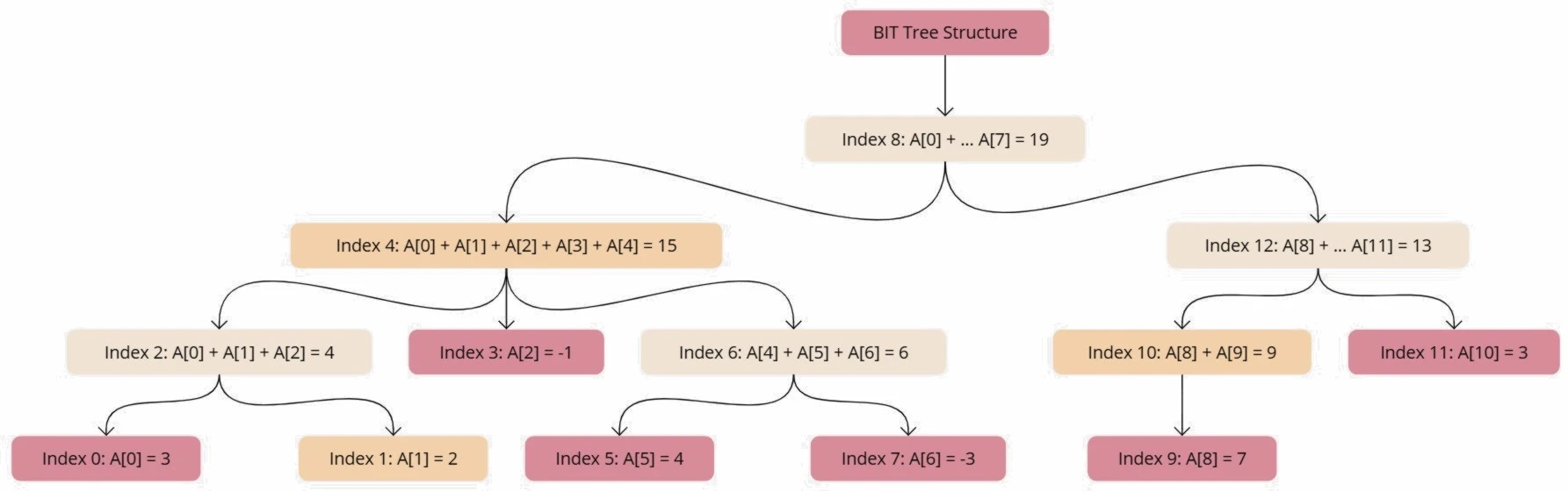 Gráfico 1.1 - Example Fenwick tree diagram.
11.7.2. Querying the Fenwick tree
When querying the sum of elements from the start of the array to index $i$, the Fenwick tree allows us to sum over non-overlapping segments by traversing the tree upwards:
Here’s the pseudocode for the sum operation:
def sum(i):
    total = 0
    while i >= 0:
        total += BIT[i]
        i -= LSB(i)
    return total
For example, to compute the sum of elements from index $0$ to $5$, we perform the following steps:
- Start at index 5. The LSB of 5 is 1, so add $A[5]$.
- Move to index 4, since $5 - \text{LSB}(5) = 4$. The LSB of 4 is 4, so add $A[0] + A[1] + A[2] + A[3] + A[4]$.
Thus, the sum of elements from index $0$ to $5$ is:
\[\text{sum}(0, 5) = \text{BIT}[5] + \text{BIT}[4] = A[5] + (A[0] + A[1] + A[2] + A[3] + A[4])\]11.7.3. Updating the Fenwick tree
When updating the value of an element in the original array, the Fenwick tree allows us to update all the relevant cumulative sums efficiently. Here’s the pseudocode for the update operation:
def update(i, delta):
    while i < len(BIT):
        BIT[i] += delta
        i += LSB(i)
For example, if we update $A[4]$, the Fenwick tree must update the sums stored at indices that cover $A[4]$’s range.
- Start at index 4. Add the change to $\text{BIT}[4]$.
- Move to index 8 and update $\text{BIT}[8]$.
In each case, the number of operations required is proportional to the number of set bits in the index, which guarantees that both update and query operations run in $O(\log n)$.
11.7.4. Basic Operations
Update
To update an element at position $i$, we traverse the tree as follows:
void update(int i, int delta) {
    for (; i < n; i += i & (-i)) {
        BIT[i] += delta;
    }
}
[Image placeholder] Illustrate the update process, showing how the Fenwick tree array is updated step by step using the least significant bit.
4.2 Prefix Sum Query
To compute the sum of elements from 0 to $i$:
int query(int i) {
    int sum = 0;
    for (; i >= 0; i -= i & (-i)) {
        sum += BIT[i];
    }
    return sum;
}
[Image placeholder] Visualize the prefix sum query operation, showing how the Fenwick tree is traversed from $i$ down to 0 using the least significant bit.
4.3 Range Query
To compute the sum of elements in the range $[l, r]$:
int rangeQuery(int l, int r) {
    return query(r) - query(l - 1);
}
5. Fenwick tree Construction
The Fenwick tree can be constructed in $O(n)$ time using the following technique:
vector<int> constructBIT(const vector<int>& arr) {
    int n = arr.size();
    vector<int> BIT(n, 0);
    for (int i = 0; i < n; i++) {
        int idx = i;
        BIT[idx] += arr[i];
        int parent = idx + (idx & (-idx));
        if (parent < n) {
            BIT[parent] += BIT[idx];
        }
    }
    return BIT;
}
[Image placeholder] An illustration that explains how the Fenwick tree is constructed from an array, showing the incremental process of building the tree.
Complexity Analysis
- Construction: $O(n)$
- Update: $O(\log n)$
- Query: $O(\log n)$
- Space: $O(n)$
Variations and Extensions
Range Update and Point Query
It is possible to modify the Fenwick tree to support range updates and point queries:
void rangeUpdate(int l, int r, int val) {
    update(l, val);
    update(r + 1, -val);
}

int pointQuery(int i) {
    return query(i);
}
Range Update and Range Query
To support both range updates and range queries, we need two Fenwick trees:
void rangeUpdate(int l, int r, int val) {
    update(BIT1, l, val);
    update(BIT1, r + 1, -val);
    update(BIT2, l, val * (l - 1));
    update(BIT2, r + 1, -val * r);
}

int prefixSum(int i) {
    return query(BIT1, i) * i - query(BIT2, i);
}

int rangeQuery(int l, int r) {
    return prefixSum(r) - prefixSum(l - 1);
}
2D Fenwick tree
The Fenwick tree can be extended to two dimensions:
void update2D(int x, int y, int delta) {
    for (int i = x; i < n; i += i & (-i))
        for (int j = y; j < m; j += j & (-j))
            BIT[i][j] += delta;
}

int query2D(int x, int y) {
    int sum = 0;
    for (int i = x; i >= 0; i -= i & (-i))
        for (int j = y; j >= 0; j -= j & (-j))
            sum += BIT[i][j];
    return sum;
}
[Image placeholder] A diagram illustrating how a 2D Fenwick tree operates, showing how updates and queries are performed in two dimensions.
Applications
- Efficient computation of prefix sums in mutable arrays
- Counting inversions in an array
- Solving the “k-th smallest element” problem
- Implementation of arithmetic coding algorithm
Comparison with Other Structures
| Structure | Update | Query | Space |
|---|---|---|---|
| Array | $O(1)$ | $O(n)$ | $O(n)$ |
| Prefix Sum | $O(n)$ | $O(1)$ | $O(n)$ |
| Segment Tree | $O(\log n)$ | $O(\log n)$ | $O(n)$ |
| Fenwick tree | $O(\log n)$ | $O(\log n)$ | $O(n)$ |
The Fenwick tree offers a good balance between update and query efficiency, with a simpler implementation than a Segment Tree.
Problem Example: “Humidity Levels in a Greenhouse” (Problem 1)
The same problem we saw earlier in the section: Algorithm: Difference Array - Efficient Range Updates. Below is the implementation in C++20:
I chose to write this code using as much modern C++ as possible. This means you will face two challenges. The first is understanding the Fenwick tree algorithm, and the second is understanding the C++ syntax. To help make this easier, I will explain the code block by block, highlighting each C++ feature and why I chose to write it this way.
Code 4:
#include <iostream>
#include <vector>
#include <numeric>
#include <fstream>
#include <sstream>
#include <filesystem>
#include <syncstream>

using namespace std;
namespace fs = filesystem;

namespace config {
    enum class InputMethod { Hardcoded, Stdin, File };

    // Altere esta linha para mudar o método de entrada
    inline constexpr InputMethod input_method = InputMethod::Hardcoded;
}

using vi = vector<int>;
using vvi = vector<vector<int>>;
using vll = vector<long long>;

class BIT {
    vi tree;
    int n;

public:
    Fenwick tree(int size) : tree(size + 1), n(size) {}

    void update(int i, int delta) {
        for (++i; i <= n; i += i & -i) tree[i] += delta;
    }

    long long query(int i) const {
        long long sum = 0;
        for (++i; i > 0; i -= i & -i) sum += tree[i];
        return sum;
    }
};

vll adjustHumidity(vi& humidity, const vvi& adjustments) {
    int n = humidity.size();
    BIT bit(n);
    vll result;
    result.reserve(adjustments.size());

    auto updateBit = [&](int i, int old_val, int new_val) {
        if (!(old_val & 1)) bit.update(i, -old_val);
        if (!(new_val & 1)) bit.update(i, new_val);
        };

    for (int i = 0; i < n; ++i) {
        if (!(humidity[i] & 1)) bit.update(i, humidity[i]);
    }

    for (const auto& adj : adjustments) {
        int i = adj[1], old_val = humidity[i], new_val = old_val + adj[0];
        updateBit(i, old_val, new_val);
        humidity[i] = new_val;
        result.push_back(bit.query(n - 1));
    }

    return result;
}

void printResult(osyncstream& out, const vi& humidity, const vvi& adjustments, const vll& result) {
    out << "**Input**: humidity = [" << humidity[0];
    for (int i = 1; i < humidity.size(); ++i) out << ", " << humidity[i];
    out << "], adjustments = [";
    for (const auto& adj : adjustments)
        out << "[" << adj[0] << "," << adj[1] << "]" << (&adj != &adjustments.back() ? ", " : "");
    out << "]\n**Output**: ";
    for (auto res : result) out << res << " ";
    out << "\n\n";
}

pair<vi, vvi> readInput(istream& in) {
    vi humidity;
    vvi adjustments;
    int n, m;
    in >> n;
    humidity.resize(n);
    for (int& h : humidity) in >> h;
    in >> m;
    adjustments.resize(m, vi(2));
    for (auto& adj : adjustments) in >> adj[0] >> adj[1];
    return { humidity, adjustments };
}

void processInput(istream& in, osyncstream& out) {
    int t;
    in >> t;
    for (int i = 1; i <= t; ++i) {
        out << "Example " << i << ":\n";
        auto [humidity, adjustments] = readInput(in);
        auto result = adjustHumidity(humidity, adjustments);
        printResult(out, humidity, adjustments, result);
    }
}

int main() {
    osyncstream syncout(cout);

    if constexpr (config::input_method == config::InputMethod::Hardcoded) {
        vector<pair<vi, vvi>> tests = {{{45, 52, 33, 64}, {{5,0}, {-20,1}, {-14,0}, {18,3}}},{{40}, {{12,0}}},{{30, 41, 55, 68, 72}, {{10,0}, {-15,2}, {22,1}, {-8,4}, {5,3}}}};

        for (int i = 0; i < tests.size(); ++i) {
            syncout << "Example " << i + 1 << ":\n";
            auto& [humidity, adjustments] = tests[i];
            auto result = adjustHumidity(humidity, adjustments);
            printResult(syncout, humidity, adjustments, result);
        }
    }
    else if constexpr (config::input_method == config::InputMethod::Stdin) {
        processInput(cin, syncout);
    }
    else if constexpr (config::input_method == config::InputMethod::File) {
        fs::path inputPath = "input.txt";
        if (fs::exists(inputPath)) {
            ifstream inputFile(inputPath);
            processInput(inputFile, syncout);
        }
        else {
            syncout << "Input file not found: " << inputPath << endl;
        }
    }
    else {
        syncout << "Invalid input method defined" << endl;
    }

    return 0;
}
The first thing you should notice is that I chose to include all three possible input methods in the same code. Obviously, in a competition, you wouldn’t do that. You would include only the method that interests you. Additionally, I opted to use modern C++20 capabilities instead of using the old preprocessor directives (#defines). However, before diving into the analysis of Code 4, let’s look at an example of what the main function would look like if we were using preprocessor directives.
#include ...

// Define input methods
#define INPUT_HARDCODED 1
#define INPUT_STDIN 2
#define INPUT_FILE 3

// Select input method here
#define INPUT_METHOD INPUT_STDIN

// lot of code goes here

int main() {
    // Creates a synchronized output stream (osyncstream) to ensure thread-safe output to cout.
    osyncstream syncout(cout);

    // Check if the input method is defined as INPUT_HARDCODED using preprocessor directives.
#if INPUT_METHOD == INPUT_HARDCODED
    // Define a vector of pairs where each pair contains:
    // 1. A vector of humidity levels.
    // 2. A 2D vector representing adjustments (value, index) to be applied to the humidity levels.

    vector<pair<vi, vvi>> tests = {
        {{45, 52, 33, 64}, {{5,0}, {-20,1}, {-14,0}, {18,3}}},
        {{40}, {{12,0}}},
        {{30, 41, 55, 68, 72}, {{10,0}, {-15,2}, {22,1}, {-8,4}, {5,3}}}
    };

    // Iterate over each hardcoded test case.
    for (int i = 0; i < tests.size(); ++i) {
        // Print the example number using synchronized output to avoid race conditions in a multithreaded context.
        syncout << "Example " << i + 1 << ":\n";

        // Extract the humidity vector and adjustments vector using structured bindings (C++17 feature).
        auto& [humidity, adjustments] = tests[i];

        // Call the adjustHumidity function to apply the adjustments and get the results.
        auto result = adjustHumidity(humidity, adjustments);

        // Print the humidity, adjustments, and the results using the printResult function.
        printResult(syncout, humidity, adjustments, result);
    }

    // If the input method is INPUT_STDIN, process input from standard input.
#elif INPUT_METHOD == INPUT_STDIN
    // Call processInput to read input from standard input and produce output.
    processInput(cin, syncout);

    // If the input method is INPUT_FILE, read input from a file.
#elif INPUT_METHOD == INPUT_FILE
    // Define the file path where the input data is expected.
    fs::path inputPath = "input.txt";

    // Check if the file exists at the specified path.
    if (fs::exists(inputPath)) {
        // If the file exists, open it as an input file stream.
        ifstream inputFile(inputPath);

        // Call processInput to read data from the input file and produce output.
        processInput(inputFile, syncout);
    } else {
        // If the file does not exist, print an error message indicating that the input file was not found.
        syncout << "Input file not found: " << inputPath << endl;
    }

    // If none of the above input methods are defined, print an error message for an invalid input method.
#else
    syncout << "Invalid INPUT_METHOD defined" << endl;
#endif

    // Return 0 to indicate successful program termination.
    return 0;
}
The code fragment uses preprocessor directives to switch between different input methods for reading data, based on a pre-defined configuration. This is done using #define statements at the top of the code and #if, #elif, and #else directives in the main function.
Input Method Definitions:
#define INPUT_HARDCODED 1
#define INPUT_STDIN 2
#define INPUT_FILE 3
These #define statements assign integer values to three possible input methods:
INPUT_HARDCODED: The input data is hardcoded directly into the program.INPUT_STDIN: The input data is read from standard input (stdin), such as from the console.INPUT_FILE: The input data is read from a file, typically stored on disk.
Input Method Selection:
#define INPUT_METHOD INPUT_STDIN
This line selects the input method by defining INPUT_METHOD. In this case, it is set to INPUT_STDIN, meaning that the program will expect to read input from the console. Changing this to INPUT_HARDCODED or INPUT_FILE would switch the input source.
Conditional Compilation (#if, #elif, #else):
The conditional compilation directives (#if, #elif, #else) are used to include or exclude specific blocks of code based on the value of INPUT_METHOD.
#if INPUT_METHOD == INPUT_HARDCODED
    // Code for hardcoded input goes here
#elif INPUT_METHOD == INPUT_STDIN
    // Code for reading from standard input goes here
#elif INPUT_METHOD == INPUT_FILE
    // Code for reading from a file goes here
#else
    // Code for handling invalid input method goes here
#endif
#if INPUT_METHOD == INPUT_HARDCODED: If the input method is hardcoded, a predefined set of test cases (humidity levels and adjustments) will be used.#elif INPUT_METHOD == INPUT_STDIN: If the input method is set to standard input, the program will read from the console.#elif INPUT_METHOD == INPUT_FILE: If the input method is set to file input, the program will attempt to read from a file (input.txt).#else: If an invalidINPUT_METHODis defined, an error message is printed.
These preprocessor directives enable the program to easily switch between input methods without having to manually modify the logic inside main, providing flexibility depending on how the input is expected during execution. But, since we are using C++20, this might not be the best solution. It may be the fastest for competitions, but there is a fundamental reason why I’m making things a bit more complex here. Beyond just learning how to write code for competitions, we are also learning C++20. Let’s start by:
The code starts by importing the std namespace globally with using namespace std;, which allows using standard C++ objects (like cout, vector, etc.) without having to prefix them with std::.
s
using namespace std; // Use the standard namespace to avoid typing "std::" before standard types.
The line namespace fs = filesystem; creates an alias for the filesystem namespace, allowing the code to reference filesystem functions more concisely, using fs:: instead of std::filesystem::.
namespace fs = filesystem; // Alias for the filesystem namespace.
Inside the config namespace, there is an enum class InputMethod that defines three possible input methods: Hardcoded, Stdin, and File. This helps manage how input will be provided to the program.
namespace config {
    enum class InputMethod { Hardcoded, Stdin, File };  // Enum to define input methods
The
namespace configis used to encapsulate related constants and configuration settings into a specific scope. In this case, it organizes the input methods and settings used in the program. By placing these within a namespace, we avoid cluttering the global namespace, ensuring that these settings are logically grouped together. This encapsulation makes it easier to maintain the code, preventing potential naming conflicts and allowing future expansion of the configuration without affecting other parts of the program.The
namespace configdoes not come from the standard C++ library; it is created specifically within this code to group configurations like theInputMethod. The use of namespaces in C++ allows developers to organize code and avoid naming conflicts but is independent of the C++ Standard Library or language itself.The
enum class InputMethodprovides a strongly typed, scoped enumeration. Unlike traditional enums, anenum classdoes not implicitly convert its values to integers, which helps prevent accidental misuse of values. The scoped nature ofenum classalso means that its values are contained within the enumeration itself, avoiding naming conflicts with other parts of the program. For instance, instead of directly usingHardcoded, you useInputMethod::Hardcoded, making the code more readable and avoiding ambiguity.Here’s an example of using an enum class in a small program. This example demonstrates how to select an input method based on the defined
InputMethod:#include <iostream> enum class InputMethod { Hardcoded, Stdin, File }; void selectInputMethod(InputMethod method) { switch (method) { case InputMethod::Hardcoded: std::cout << "Using hardcoded input.\n"; break; case InputMethod::Stdin: std::cout << "Reading input from stdin.\n"; break; case InputMethod::File: std::cout << "Reading input from a file.\n"; break; } } int main() { InputMethod method = InputMethod::File; selectInputMethod(method); // **Output**: Reading input from a file. return 0; }In this example, the
enum class InputMethodallows for a clear, type-safe way to represent the input method, making the code easier to manage and less error-prone.
The inline constexpr constant input_method specifies which input method will be used by default. In this case, it is set to InputMethod::Hardcoded, meaning the input will be predefined inside the code. The inline constexpr allows the value to be defined at compile time, making it a more efficient configuration option.
    inline constexpr InputMethod input_method = InputMethod::Hardcoded;  // Default input method is hardcoded.
}
The
inlinekeyword in C++ specifies that a function, variable, or constant is defined inline, meaning the compiler should attempt to replace function calls with the actual code of the function. This can improve performance by avoiding the overhead of a function call. However, the main use ofinlinein modern C++ is to avoid the “multiple definition” problem when defining variables or functions in header files that are included in multiple translation units.inline int square(int x) { return x * x; // This function is defined inline, so calls to square(3) may be replaced with 3 * 3 directly. }When
inlineis used with variables or constants, it allows those variables or constants to be defined in a header file without violating the One Definition Rule (ODR). Each translation unit that includes the header will have its own copy of the inline variable, but the linker will ensure that only one copy is used in the final binary.inline constexpr int max_value = 100; // This constant can be included in multiple translation units without causing redefinition errors.The
constexprkeyword specifies that a function or variable can be evaluated at compile-time. It guarantees that, if possible, the function will be computed by the compiler, not at runtime. This is especially useful in optimization, as it allows constants to be determined and used during the compilation process rather than execution.
constexprwith Variables: When you useconstexprwith variables, the compiler knows that the variable’s value is constant and should be computed at compile time.constexpr int max_items = 42; // The value of max_items is known at compile-time and cannot change.You can use
constexprvariables to define array sizes or template parameters because their values are known during compilation.constexpr int size = 10; int array[size]; // Valid, because size is a constant expression.
constexprwith Functions: Aconstexprfunction is a function whose return value can be computed at compile time if the inputs are constant expressions. The function must have a single return statement and all operations within it must be valid at compile time.constexpr int factorial(int n) { return n <= 1 ? 1 : n * factorial(n - 1); // Recursive function that computes the factorial at compile time. }If
factorial(5)is called with a constant value, the compiler will compute the result at compile time and replace the function call with120in the generated binary. ? Combininginlineandconstexpr: A function can be bothinlineandconstexpr, which means the function can be evaluated at compile time and its calls may be inlined if appropriate.inline constexpr int power(int base, int exp) { return (exp == 0) ? 1 : base * power(base, exp - 1); }In this case, the
powerfunction will be inlined when called at runtime and computed at compile time if the arguments are constant. For example,power(2, 3)would be replaced by8at compile time.Practical Use of
constexpr:constexprcan be used in a wide variety of contexts, such as constructing constant data, optimizing algorithms, and defining efficient compile-time logic. Here are a few examples:
- Compile-time array size:
constexpr int size = 5;
int array[size];  // The size is computed at compile time.
- Compile-time strings:
constexpr const char* greet() { return "Hello, World!"; }
constexpr const char* message = greet();  // The message is computed at compile time.
- Compile-time mathematical operations:
constexpr int area(int length, int width) {
    return length * width;
}
constexpr int room_area = area(10, 12);  // Computed at compile time.
Using
constexprin Competitive Programming: In competitive programming,constexprcan be both an advantage and a disadvantage, depending on how it is used.
Advantage:
constexprcan optimize code by computing results at compile time rather than runtime, which can save valuable processing time. For example, if you know certain values or calculations are constant throughout the competition, you can useconstexprto precompute them, thereby avoiding recalculations during execution.Disadvantage: However, in many competitive programming problems, the input is dynamic and provided at runtime, meaning that
constexprcannot be used for computations that depend on this input. Since the focus in competitive programming is on runtime efficiency, the use ofconstexpris limited to cases where you can precompute values before the competition or during compilation.Overall,
constexpris valuable when solving problems with static data or fixed input sizes, but in typical ICPC-style competitions, its usage may be less frequent because most problems require dynamic input processing.In summary,
inlinehelps with reducing overhead by allowing the compiler to replace function calls with the actual function code, and it prevents multiple definitions of variables in multiple translation units.constexprenables computations to be performed at compile time, which can significantly optimize performance by avoiding runtime calculations, although its applicability in competitive programming may be limited.
AINDA TEM MUITO QUE EXPLICAR AQUI.
Inventory Restocking
You manage a warehouse where products are stored and moved frequently. The warehouse tracks its inventory by recording the stock count at different times during the day in an array $inventory$. Occasionally, inventory managers report the amount by which a product’s stock needs to be adjusted, represented by an integer array $adjustments$, where each adjustment is a pair $[adjustment, index]$. Your task is to apply these adjustments and after each, calculate the total count of products with even stock numbers.
Input Format:
- The first line contains an integer $n$, representing the size of the $inventory$ array.
- The second line contains $n$ integers representing the initial values in the $inventory$ array.
- The third line contains an integer $q$, the number of stock adjustments.
- The following $q$ lines each contain a pair $adjustment$ and $index$, where $adjustment$ is the amount to be added or subtracted, and $index$ is the position in the $inventory$ array to adjust.
Constraints:
- $1 \leq n, q \leq 10^5$
- $-10^4 \leq inventory[i], adjustment \leq 10^4$
Example **Input:**
6
10 3 5 6 8 2
4
[3, 1]
[-4, 0]
[2, 3]
[-3, 4]
Example **Output:**
26
16
20
16
Explanation:
Initially, the array is $[10, 3, 5, 6, 8, 2]$, and the sum of even values is $10 + 6 + 8 + 2 = 26$.
- After adding $3$ to $inventory[1]$, the array becomes $[10, 6, 5, 6, 8, 2]$, and the sum of even values is $10 + 6 + 6 + 8 + 2 = 32$.
- After subtracting $4$ from $inventory[0]$, the array becomes $[6, 6, 5, 6, 8, 2]$, and the sum of even values is $6 + 6 + 6 + 8 + 2 = 28$.
Input Method:
The input will be provided via hardcoded values inside the code for testing purposes.
Naïve Solution
- Initially, the even numbers in $inventory$ are $10$, $6$, $8$, $2$. The sum of these values is $26$.
- After the first adjustment $[3, 1]$, the inventory becomes $[10, 6, 5, 6, 8, 2]$. The even numbers are now $10$, $6$, $8$, $2$. The sum remains $26$.
- After the second adjustment $[-4, 0]$, the inventory becomes $[6, 6, 5, 6, 8, 2]$. The even numbers are $6$, $6$, $8$, $2$. The sum is $16$.
- After the third adjustment $[2, 3]$, the inventory becomes $[6, 6, 5, 8, 8, 2]$. The even numbers are $6$, $6$, $8$, $8$, $2$. The sum is $20$.
- After the fourth adjustment $[-3, 4]$, the inventory becomes $[6, 6, 5, 8, 5, 2]$. The even numbers are $6$, $6$, $8$, $2$. The sum is $16$.
Pseudo Code Solution using python:
Here is a Python solution that solves the problem as simply and directly as requested:
# Read the size of the inventory array
n = int(input())

# Read the inventory array
inventory = list(map(int, input().split()))

# Read the number of adjustments
q = int(input())

# Initialize the sum of even numbers
even_sum = sum([x for x in inventory if x % 2 == 0])

# Process the adjustments
for _ in range(q):
    adjustment, index = map(int, input().strip('[]').split(','))

    # Check if the current value at the index is even before the adjustment
    if inventory[index] % 2 == 0:
        even_sum -= inventory[index]  # Remove from the sum if it was even

    # Apply the adjustment
    inventory[index] += adjustment

    # Check if the new value at the index is even after the adjustment
    if inventory[index] % 2 == 0:
        even_sum += inventory[index]  # Add to the sum if it is now even

    # Print the updated sum of even numbers
    print(even_sum)
In this pseudocode, we observe the following steps:
- Input Reading: First, we read the value of $n$ (inventory size) and the integer array $inventory$. Then, we read the number of adjustments $q$ and each adjustment.
- Initial Calculation: We calculate the initial sum of even numbers in the $inventory$ array.
- Processing Adjustments: For each adjustment, we check if the value at the affected index is even before the adjustment. If it is, we remove that value from the sum of even numbers. We then apply the adjustment, and if the new value at the index is even, we add it to the sum of even numbers.
- Output: After each adjustment, we print the updated sum of even numbers.
For this solution the time complexity is $O(n + q)$, where $n$ is the size of the $inventory$ array and $q$ is the number of adjustments. The code processes each adjustment in constant time since the sum is maintained incrementally.
#include <iostream>
#include <vector>

using namespace std;

int main() {
    // Hardcoded input values
    int n = 6, q = 4;
    vector<int> inventory = { 10, 3, 5, 6, 8, 2 };
    vector<pair<int, int>> adjustments = { {3, 1}, {-4, 0}, {2, 3}, {-3, 4} };

    // Initial sum of even numbers
    int even_sum = 0;
    for (int i = 0; i < n; ++i)
        if (!(inventory[i] & 1)) even_sum += inventory[i]; // Check if even

    // Process adjustments
    for (int i = 0; i < q; ++i) {
        int adj = adjustments[i].first, idx = adjustments[i].second;
        if (!(inventory[idx] & 1)) even_sum -= inventory[idx]; // Subtract if even
        inventory[idx] += adj;  // Apply adjustment
        if (!(inventory[idx] & 1)) even_sum += inventory[idx]; // Add if now even
        cout << even_sum << '\n';
    }
}
In C++, the expression
inventory[i] & 1is a bitwise operation that checks whether the value at index $i$ in theinventoryarray is even or odd.
Detailed Explanation:
&Operator: This is the bitwise AND operator. It performs an AND operation on the binary representation of two numbers, comparing corresponding bits.1in Binary: The number $1$ in binary is represented as $0000…0001$ (depending on the size of the integer). Since only the least significant bit is set to $1$, this operation focuses specifically on the least significant bit ofinventory[i].- Bitwise AND (
&): The bitwise AND operator returns $1$ if both corresponding bits of the operands are $1$. For other cases, it returns $0$.
In the naïve code this operation checks whether the least significant bit (LSB) of the value at inventory[i] is $1$ or $0$, which directly indicates if the number is odd or even:
- If the result of
inventory[i] & 1is $1$, the number is odd. - If the result of
inventory[i] & 1is $0$, the number is even.
This bitwise approach is faster than using the modulo operation (inventory[i] % 2 == 0) for determining even/odd status, as it avoids division and is optimized at the hardware level. Consider the following values for inventory[i]:
- For
inventory[i] = 6(binary: $110$), the operation:- $6 \& 1 = 0$
- Since the result is $0$, 6 is even.
-
For
inventory[i] = 5(binary: $101$), the operation:- $5 \& 1 = 1$
- Since the result is $1$, 5 is odd.
Bitwise Operations in C++
Bitwise operations in C++ manipulate individual bits of integers. These operations are low-level but powerful, allowing programmers to perform tasks like toggling, setting, or clearing specific bits. They are commonly used in scenarios where performance is critical, such as embedded systems, cryptography, and competitive programming.
C++ provides several bitwise operators that work directly on the binary representation of numbers. These operators include:
- AND (
&)- OR (
|)- XOR (
^)- NOT (
~)- Left Shift (
<<)- Right Shift (
>>)Bitwise AND (
&)The bitwise AND operator compares each bit of its operands and returns $1$ if both bits are $1$. Otherwise, it returns $0$.
int a = 6;    // Binary: 110
int b = 3;    // Binary: 011
int result = a & b;  // result = 2 (Binary: 010)
In this code we have: the binary representation of 6 is $110$ and the binary representation of 3 is $011$. When performing the AND operation:
- $1 \& 0 = 0$
- $1 \& 1 = 1$
- $0 \& 1 = 0$
Therefore, the result is $010$ in binary, which is $2$ in decimal.
Bitwise OR (
|)The bitwise OR operator compares each bit of its operands and returns $1$ if either of the bits is $1$.
int a = 6;    // Binary: 110
int b = 3;    // Binary: 011
int result = a | b;  // result = 7 (Binary: 111)
The binary representation of 6 is $110$ and the binary representation of 3 is $011$. When performing the OR operation:
- $1 | 0 = 1$
- $1 | 1 = 1$
- $0 | 1 = 1$
Therefore, the result is $111$ in binary, which is $7$ in decimal.
Bitwise XOR (
^)The bitwise XOR (exclusive OR) operator compares each bit of its operands and returns $1$ if the bits are different, and $0$ if they are the same.
int a = 6;    // Binary: 110
int b = 3;    // Binary: 011
int result = a ^ b;  // result = 5 (Binary: 101)
The binary representation of 6 is $110$ and the binary representation of 3 is $011$. When performing the XOR operation:
- $1 \oplus 0 = 1$
- $1 \oplus 1 = 0$
- $0 \oplus 1 = 1$
- Therefore, the result is $101$ in binary, which is $5$ in decimal.
Bitwise NOT (
~)The bitwise NOT operator inverts all the bits of its operand. It converts $1$s to $0$s and $0$s to $1$s.
int a = 6;    // Binary: 00000000 00000000 00000000 00000110 (32-bit system)
int result = ~a;  // result = -7 (Binary: 11111111 11111111 11111111 11111001)
The binary representation of 6 is $0000…0110$ (with 32 bits). The NOT operation flips each bit: $~110$ becomes $111…1001$.The result is the two’s complement representation of $-7$.
Left Shift (
<<)The left shift operator shifts the bits of its first operand to the left by the number of positions specified by the second operand. This effectively multiplies the number by powers of 2.
int a = 3;    // Binary: 00000000 00000000 00000000 00000011
int result = a << 1;  // result = 6 (Binary: 00000000 00000000 00000000 00000110)
The binary representation of 3 is $011$. Shifting it left by $1$ position results in $110$, which is $6$ in decimal. Shifting by $n$ positions is equivalent to multiplying by $2^n$.
Right Shift (
>>)The right shift operator shifts the bits of its first operand to the right by the number of positions specified by the second operand. This effectively divides the number by powers of 2 (for positive integers).
int a = 6;    // Binary: 00000000 00000000 00000000 00000110
int result = a >> 1;  // result = 3 (Binary: 00000000 00000000 00000000 00000011)
The binary representation of 6 is $110$. Shifting it right by $1$ position results in $011$, which is $3$ in decimal.Shifting by $n$ positions is equivalent to dividing by $2^n$ (for non-negative integers).
Summary Table of Bitwise Operations
Operation Symbol Effect Bitwise AND &Compares bits, returns $1$ if both are $1$. Bitwise OR ` ` Compares bits, returns $1$ if at least one is $1$. Bitwise XOR ^Compares bits, returns $1$ if bits are different. Bitwise NOT ~Inverts each bit (turns $0$s into $1$s and $1$s into $0$s). Left Shift <<Shifts bits to the left, multiplying by powers of 2. Right Shift >>Shifts bits to the right, dividing by powers of 2 (for positive numbers). Applications of Bitwise Operations:
- Efficiency: Bitwise operations are faster than arithmetic operations, making them useful in performance-critical code.
- Bit Manipulation: They are commonly used for tasks such as toggling, setting, and clearing bits in low-level programming, such as working with hardware or network protocols.
- Masking and Flagging: Bitwise operators are often used to manipulate flags in bitmasks, where individual bits represent different conditions or options.
4 - Sales Target Analysis
You are tasked with analyzing sales data to determine how many subarrays of daily sales sum to a multiple of a target value $T$ . The sales data is recorded in an array sales , and you need to calculate how many contiguous subarrays of sales have a sum divisible by $T$ .
Input Format:
The first line contains two integers $n$ (the size of the sales array) and $T$ (the target value). The second line contains $n$ integers, representing the daily sales data. Constraints:
\[1 \leq n \leq 10^5 \\ 1 \leq T \leq 10^4 \\ -10^4 \leq \text{sales}[i] \leq 10^4\]Output Format:
Output a single integer representing the number of subarrays whose sum is divisible by $T$ .
Example Input: 6 5 4 5 0 -2 -3 1
Example Output: 7
Explanation:
There are $7$ subarrays whose sum is divisible by $T=5$ :
[4,5,0,−2,−3,1]
[5]
[5,0]
[5,0,−2,−3]
[0]
[0,−2,−3]
[−2,−3]
Input Method:
The input is provided via command-line arguments.
Naïve Code
The algorithm works as follows:
-
We define a function
count_divisible_subarraysthat takes thesalesarray and target valueTas inputs. -
We use two nested loops to generate all possible subarrays:
- The outer loop (
start) determines the starting index of each subarray. - The inner loop (
end) determines the ending index of each subarray.
- The outer loop (
-
For each subarray, we calculate the sum (
subarray_sum) and check if it’s divisible byT. -
If a subarray sum is divisible by
T, we increment ourcount. -
After checking all subarrays, we return the total
count. -
Outside the function, we read the input from command-line arguments:
nandTare the first two arguments.- The
salesarray is constructed from the remaining arguments.
-
We call our function with the input data and print the result.
Here’s a simple algorithm to solve the Sales Target Analysis problem, described in English with Python as pseudo-code:
-
Define a function to count divisible subarrays:
def count_divisible_subarrays(sales, T): count = 0 for start in range(len(sales)): subarray_sum = 0 for end in range(start, len(sales)): subarray_sum += sales[end] if subarray_sum % T == 0: count += 1 return count -
Read input from command-line arguments:
n, T = map(int, sys.argv[1:3]) sales = list(map(int, sys.argv[3:])) -
Call the function and print the result:
result = count_divisible_subarrays(sales, T)
print(result)
The time complexity of this algorithm is $O(n^2)$, where $n$ is the number of elements in the sales array. This is because we’re checking all possible subarrays, which requires two nested loops.
While this solution is straightforward and works for small inputs, it may not be efficient for large datasets (up to $10^5$ elements as per the problem constraints). An optimized solution using prefix sums and modular arithmetic could solve this problem in $O(n)$ time, but that’s beyond the scope of a beginner’s approach.
#include <iostream>
#include <vector>
#include <string>

using namespace std;

int main(int argc, char* argv[]) {
    // Read n and T from command-line arguments
    int n = stoi(argv[1]);
    int T = stoi(argv[2]);

    // Read the sales data from command-line arguments
    vector<int> sales(n);
    for (int i = 0; i < n; ++i) {
        sales[i] = stoi(argv[i + 3]);
    }

    // Function to count subarrays with sum divisible by T
    int count = 0;

    // Iterate over all possible subarrays
    for (int start = 0; start < n; ++start) {
        int subarray_sum = 0;
        for (int end = start; end < n; ++end) {
            subarray_sum += sales[end];
            if (subarray_sum % T == 0) {
                count++;
            }
        }
    }

    // Output the result
    cout << count << endl;

    return 0;
}
Both
atoiandstoiare functions used in C++ to convert strings to integers, but they differ in terms of capabilities, safety, and how they handle errors.
atoi(ASCII to Integer)The
atoifunction is a legacy C-style function that converts a C-string (i.e., a character array) to an integer. It is part of the<cstdlib>header.int atoi(const char* str);
- Parameter: The function takes a single argument,
str, which is a pointer to a null-terminated C-string (an array of characters).- Return: The function returns the integer representation of the string, or
0if the conversion fails.#include <iostream> #include <cstdlib> int main() { const char* str = "12345"; int num = atoi(str); std::cout << num << std::endl; // **Output**: 12345 return 0; }
atoireads the string and converts valid characters (i.e., digits) into an integer.- If the string contains any non-numeric characters,
atoistops reading at the first invalid character and returns the number formed so far.- If the string does not contain a valid integer at all, it returns
0.Limitations:
- Error Handling:
atoidoes not provide any error checking or exception handling. If the input is invalid (e.g., an empty string or a string with non-numeric characters), it simply returns0, making it hard to detect if an error occurred.- Overflow/Underflow: There is no way to detect if the resulting integer overflows or underflows the limits of the
inttype.
stoi(String to Integer):The
stoifunction is a C++-specific function that is more robust and safer thanatoi. It is part of the<string>header and can convert astd::stringor C-string to an integer. Unlikeatoi,stoiprovides error handling and works with thestd::stringclass.int stoi(const std::string& str, size_t* idx = 0, int base = 10);
- Parameters:
str: A reference to astd::stringobject or a C-string to be converted.idx(optional): A pointer to asize_tvariable where the function stores the index of the first invalid character. If no invalid character is found, this is ignored.base(optional): The base of the number system (default is base 10). It can handle different bases like hexadecimal (base 16), octal (base 8), etc.- Return: The function returns the integer representation of the string.
- Exception: Throws
std::invalid_argumentif no conversion can be performed, orstd::out_of_rangeif the resulting integer is out of range for theinttype.#include <iostream> #include <string> int main() { std::string str = "6789"; int num = stoi(str); std::cout << num << std::endl; // **Output**: 6789 // Handling conversion with an invalid character try { std::string invalid_str = "123abc"; int invalid_num = stoi(invalid_str); // Throws an exception } catch (const std::invalid_argument& e) { std::cout << "Invalid argument: " << e.what() << std::endl; } return 0; }
stoistarts from the beginning of the string and converts as many valid numeric characters as it can into an integer.- If the string contains any non-numeric characters, the function will throw an exception (
std::invalid_argument).- If the resulting integer exceeds the bounds of the
inttype,std::out_of_rangeis thrown.Advantages:
- Error Handling: Unlike
atoi,stoiprovides proper error handling through exceptions, making it more robust.- Base Conversion:
stoican convert numbers in different bases (e.g., hexadecimal or octal) by specifying thebaseparameter.- Range Checking: It handles integer overflow/underflow and throws
std::out_of_rangeif the value is too large or too small for theinttype.Example with Base Conversion:
std::string hex_str = "1A";  // Hexadecimal string
int num = stoi(hex_str, nullptr, 16);  // Converts from base 16 (hex) to base 10
std::cout << num << std::endl;  // **Output**: 26
Summary of Differences:
Feature atoistoiInput C-string ( const char*)std::stringor C-stringError Handling Returns 0for invalid inputThrows std::invalid_argumentorstd::out_of_rangeBase Conversion Only base 10 Supports multiple bases Exception Safety No Yes (uses C++ exceptions) Overflow/Underflow No handling Detects and throws std::out_of_range
Search and Sorting Algorithms
Binary Search
Problems that require efficient lookup in a sorted array or determining a condition within a range can be solved using binary search with time complexity $O(\log n)$.
Sorting
Sorting problems involve ordering data to simplify subsequent tasks. Efficient sorting algorithms, such as mergesort or quicksort, run in $O(n \log n)$ time and are frequently needed as a preprocessing step for more complex algorithms.
Data Structures
Stacks and Queues
Problems involving stack-based or queue-based flows, where order of insertion and removal (FIFO/LIFO) is critical, appear often.
Trees
Binary trees, AVL trees, or binary search trees (BSTs) are used in problems requiring fast insertions, deletions, and lookups. Segment trees or Fenwick trees (binary indexed trees) are commonly used for range query problems.
Priority Queues (Heaps)
Heaps are employed in problems like scheduling, dynamic sorting, or pathfinding (Dijkstra’s algorithm) to maintain a dynamic set of elements where the highest (or lowest) priority element can be accessed quickly.
Hashing
Hash maps (or dictionaries) are essential in problems requiring constant time lookups for checking membership or counting frequencies of elements.
Dynamic Programming (DP)
Knapsack Problem
Select items to maximize a total value without exceeding a capacity. Variations include 0/1 Knapsack, fractional knapsack, and bounded knapsack.
Longest Increasing Subsequence
Find the longest subsequence of a sequence where the elements are in increasing order. The time complexity can be reduced to $O(n \log n)$ using binary search in combination with dynamic programming.
Grid Pathfinding
DP-based grid traversal problems, such as finding the minimum or maximum cost path from one corner of a grid to another, often appear.
Dynamic Programming
Dynamic Programming is a different way of thinking when it comes to solving problems. Programming itself is already a different way of thinking, so, to be honest, I can say that Dynamic Programming is a different way within a different way of thinking. And, if you haven’t noticed yet, there is a concept of recursion trying to emerge in this definition.
The general idea is that you, dear reader, should be able to break a large and difficult problem into small and easy pieces. This involves storing and reusing information within the algorithm as needed.
It is very likely that you, kind reader, have been introduced to Dynamic Programming techniques while studying algorithms without realizing it. So, it is also very likely that you will encounter, in this text, algorithms you have seen before without knowing they were Dynamic Programming.
My intention is to break down the Dynamic Programming process into clear steps, focusing on the solution algorithm, so that you can understand and implement these steps on your own whenever you face a problem in technical interviews, production environments, or programming competitive programmings. Without any hesitation, I will try to present performance tips and tricks in C++. However, this should not be considered a limitation; we will prioritize understanding the algorithms before diving into the code, and you will be able to implement the code in your preferred programming language.
I will be using functions for all the algorithms I study primarily because it will make it easier to measure and compare the execution time of each one, even though I am aware of the additional computational overhead associated with function calls. After studying the problems in C++ and identifying the solution with the lowest complexity, eventually, we will also explore the best solution in C. Additionally, whenever possible, we will examine the most popular solution for the problem in question that I can find online.
Some say that Dynamic Programming is a technique to make recursive code more efficient. If we look at Dynamic Programming, we will see an optimization technique that is based on recursion but adds storage of intermediate results to avoid redundant calculations. Memoization and tabulation are the two most common Dynamic Programming techniques, each with its own approach to storing and reusing the results of subproblems:
- Memoization (Top-Down): This technique is recursive in nature. It involves storing the results of expensive function calls and returning the cached result when the same inputs occur again. This approach can be seen as an optimization of the top-down recursive process.
- Tabulation (Bottom-Up): Tabulation takes an iterative approach, solving smaller subproblems first and storing their solutions in a table (often an array or matrix). It then uses these stored values to calculate the solutions to larger subproblems, gradually building up to the final solution. The iterative nature of tabulation typically involves using loops to fill the table in a systematic manner.
Throughout our exploration of Dynamic Programming concepts, we’ve been using Python as a form of pseudocode. Its versatility and simplicity have served us well, especially considering that many of my students are already familiar with it. Python’s readability has made it an excellent choice for introducing and illustrating algorithmic concepts. However, as we progress into more advanced territory, it’s time to acknowledge that Python, despite its strengths, isn’t the most suitable language for high-performance applications or programming competitive programmings.
With this in mind, we’re going to transition to using C++ 20 as our primary language moving forward. C++ offers superior performance, which is crucial when dealing with computationally intensive tasks often found in competitive programming scenarios. It also provides more direct control over memory management, a feature that can be essential when optimizing algorithms for speed and efficiency. Additionally, we’ll occasionally use data structures compatible with C 17 within our C++ 20 environment, ensuring a balance between modern features and broader compatibility.
For our development environment, we’ll be using Visual Studio Community Edition. This robust IDE will allow us to write, compile, and evaluate our C++ code effectively. It offers powerful debugging tools and performance profiling features, which will become increasingly valuable as we delve into optimizing our algorithms.
Despite this shift, we won’t be discarding the work we’ve done so far. To maintain consistency and provide a bridge between our previous discussions and this new approach, I’ll be converting the functions we originally wrote in Python to C++.
As we make this transition, we’ll gradually introduce C++ specific optimizations and techniques, broadening your understanding of Dynamic Programming implementation across different language paradigms. I hope this approach will equip you with both a solid conceptual foundation and the practical skills needed for high-performance coding.
Example 4: Fibonacci in C++ using std::vectors:
Let’s begin with a straightforward, naive implementation in C++20.
#include <iostream>
#include <unordered_map>
#include <vector>
#include <chrono>
#include <functional>

// Recursive function to calculate Fibonacci
int fibonacci(int n) {
    if (n <= 1) {
        return n;
    }
    else {
        return fibonacci(n - 1) + fibonacci(n - 2);
    }
}

// Recursive function with memoization to calculate Fibonacci
int fibonacci_memo(int n, std::unordered_map<int, int>& memo) {
    if (memo.find(n) != memo.end()) {
        return memo[n];
    }
    if (n <= 1) {
        return n;
    }
    memo[n] = fibonacci_memo(n - 1, memo) + fibonacci_memo(n - 2, memo);
    return memo[n];
}

// Iterative function with tabulation to calculate Fibonacci
int fibonacci_tabulation(int n) {
    if (n <= 1) {
        return n;
    }
    std::vector<int> dp(n + 1, 0);
    dp[1] = 1;
    for (int i = 2; i <= n; ++i) {
        dp[i] = dp[i - 1] + dp[i - 2];
    }
    return dp[n];
}

// Function to measure execution time
template <typename Func, typename... Args>
long long measure_time(Func func, Args&&... args) {
    auto start = std::chrono::high_resolution_clock::now();
    func(std::forward<Args>(args)...);
    auto end = std::chrono::high_resolution_clock::now();
    std::chrono::duration<long long, std::nano> duration = end - start;
    return duration.count();
}

// Function to calculate average execution time
template <typename Func, typename... Args>
long long average_time(Func func, int iterations, Args&&... args) {
    long long total_time = 0;
    for (int i = 0; i < iterations; ++i) {
        total_time += measure_time(func, std::forward<Args>(args)...);
    }
    return total_time / iterations;
}

int main() {

    const int iterations = 1000;
    std::vector<int> test_cases = { 10, 20, 30 };

    for (int n : test_cases) {
        std::cout << "Calculating Fibonacci(" << n << ")\n";

        // Calculation and average time using the simple recursive function
        long long avg_time_recursive = average_time(fibonacci, iterations, n);
        std::cout << "Average time for recursive Fibonacci: " << avg_time_recursive << " ns\n";

        // Calculation and average time using the memoization function
        std::unordered_map<int, int> memo;
        auto fibonacci_memo_wrapper = [&memo](int n) { return fibonacci_memo(n, memo); };
        long long avg_time_memo = average_time(fibonacci_memo_wrapper, iterations, n);
        std::cout << "Average time for memoized Fibonacci: " << avg_time_memo << " ns\n";

        // Calculation and average time using the tabulation function
        long long avg_time_tabulation = average_time(fibonacci_tabulation, iterations, n);
        std::cout << "Average time for tabulated Fibonacci: " << avg_time_tabulation << " ns\n";

        std::cout << "-----------------------------------\n";
    }

    return 0;
}
Code 1 - Running std::vector and tail recursion
The Code 1 demonstrates not only our Fibonacci functions but also two functions for calculating execution time (long long measure_time(Func func, Args&&... args) and long long measure_time(Func func, Args&&... args)). From this point forward, I will be using this code model to maintain consistent computational cost when calculating the average execution time of the functions we create. This approach will ensure that our performance measurements are standardized across different implementations, allowing for more accurate comparisons as we explore various Dynamic Programming techniques.
Now, the attentive reader will agree with me: we must to break this code down.
The Recursive Function
Let’s start with fibonacci(int n), the simple and pure tail recursive function.
int fibonacci(int n) {
    if (n <= 1) {
        return n;
    }
    else {
        return fibonacci(n - 1) + fibonacci(n - 2);
    }
}
Code Fragment 1A - C++ Tail Recursion Function
This is a similar C++ recursive function to the one we used to explain recursion in Python. Perhaps the most relevant aspect of fibonacci(int n) is its argument: int n. Using the int type limits our Fibonacci number to $46$. Especially because the int type on my system, a 64-bit computer running Windows 11, is limited, by default, to storing a maximum value of $2^31 - 1 = 2,147,483,647$, and the $46$th Fibonacci number is $1,836,311,903$. The 47th Fibonacci number will be bigger will be bigger than int capacity.
The next function is the C++ memoization version:
The Dynamic Programming Function Using Memoization
// Recursive function with memoization to calculate Fibonacci
int fibonacci_memo(int n, std::unordered_map<int, int>& memo) {
    if (memo.find(n) != memo.end()) {
        return memo[n];
    }
    if (n <= 1) {
        return n;
    }
    memo[n] = fibonacci_memo(n - 1, memo) + fibonacci_memo(n - 2, memo);
    return memo[n];
}
Code Fragment 2A - C++ Memoization Function
Let’s highlight the std::unordered_map<int, int>& memo in function arguments. The argument std::unordered_map<int, int>& memo in C++ is used to pass a reference to an unordered map (hash table) that maps integers to integers. Breaking it down we will have:
std::unordered_mapis a template class provided by the C++ Standard Library (STL) that implements a hash table. The template parameters<int, int>specify that the keys and values stored in the unordered map are both integers.
The ampersand (&) indicates that the argument is a reference. This means that the function will receive a reference to the original unordered map, rather than a copy of it. Passing by reference is efficient because it avoids copying the entire map, which could be expensive in terms of time and memory, especially for large maps. Pay attention: Thanks to the use of &, all changes made to the map inside the function will affect the original map outside the function. Finally memo is the identifier of the parameter which type is std::unordered_map<int, int>.In the context of memoization (hence the name memo we used earlier), this unordered map is used to store the results of previously computed values to avoid redundant calculations.
One
unordered_mapin C++ is quite similar to Python’s dict in terms of functionality. Both provide an associative container that allows for efficient key-value pair storage and lookup. Thestd::unordered_mapis a template class and a C++ only construct implemented as a hash table. Unordered maps store key-value pairs and provide average constant-time complexity for insertion, deletion, and lookup operations, thanks to their underlying hash table structure. They grow dynamically as needed, managing their own memory, which is freed upon destruction. Unordered maps can be passed to or returned from functions by value and can be copied or assigned, performing a deep copy of all stored elements.Unlike arrays, unordered maps do not decay to pointers, and you cannot get a pointer to their internal data. Instead, unordered maps maintain an internal hash table, which is allocated dynamically by the allocator specified in the template parameter, usually obtaining memory from the freestore (heap) independently of the object’s actual allocation. This makes unordered maps efficient for fast access and manipulation of key-value pairs, though they do not maintain any particular order of the elements.
Unordered maps do not require a default constructor for stored objects and are well integrated with the rest of the STL, providing
begin()/end()methods and the usual STL typedefs. When reallocating, unordered maps rehash their elements, which involves reassigning the elements to new buckets based on their hash values. This rehashing process can involve copying or moving (in C++11 and later) the elements to new locations in memory.Rehashing, is the process used in
std::unordered_mapto maintain efficient performance by redistributing elements across a larger array when the load factor (the number of elements divided by the number of buckets) becomes too high. The rehashing process involves determining the new size, allocating a new array of buckets to hold the redistributed elements, rehashing elements by applying a hash function to each key to compute a new bucket index and inserting the elements into this new index, and finally, updating the internal state by updating internal pointers, references, and variables, and deallocating the old bucket array. Rehashing instd::unordered_mapis crucial for maintaining efficient performance by managing the load factor and ensuring that hash collisions remain manageable.
Overall, std::unordered_map is a versatile and efficient container for associative data storage, offering quick access and modification capabilities while seamlessly integrating with the C++ Standard Library and, for our purposes, very similar to Python’s dictionary
The fibonacci_memo(int n, std::unordered_map<int, int>& memo) function works just like the Python function we explained before with the same complexity, $O(n)$, for space and time. That said we can continue to fibonacci_tabulation(int n).
Memoization offers significant advantages over the simple recursive approach when implementing the Fibonacci sequence. The primary benefit is improved time complexity, reducing it from exponential $O(2^n)$ to linear $O(n)$. This optimization is achieved by storing previously computed results in a hash table (memo), eliminating redundant calculations that plague the naive recursive method. This efficiency becomes increasingly apparent for larger $n$ values, where the simple recursive method’s performance degrades exponentially, while the memoized version maintains linear time growth. Consequently, memoization allows for the computation of much larger Fibonacci numbers in practical time frames.
The Dynamic Programming Function Using Tabulation
The fibonacci_tabulation(int n), which uses a std::vector, was designed to be as similar as possible to the tabulation function we studied in Python.
// Iterative function with tabulation to calculate Fibonacci
int fibonacci_tabulation(int n) {
    if (n <= 1) {
        return n;
    }
    std::vector<int> dp(n + 1, 0);
    dp[1] = 1;
    for (int i = 2; i <= n; ++i) {
        dp[i] = dp[i - 1] + dp[i - 2];
    }
    return dp[n];
}
Code 1C - C++ Tabulation Function
The
std::vectoris a template class and a C++ only construct implemented as a dynamic array. Vectors grow and shrink dynamically, automatically managing their memory, which is freed upon destruction. They can be passed to or returned from functions by value and can be copied or assigned, performing a deep copy of all stored elements.Unlike arrays, vectors do not decay to pointers, but you can explicitly get a pointer to their data using
&vec[0]. Vectors maintain their size (number of elements currently stored) and capacity (number of elements that can be stored in the currently allocated block) along with the internal dynamic array. This internal array is allocated dynamically by the allocator specified in the template parameter, usually obtaining memory from the freestore (heap) independently of the object’s actual allocation. Although this can make vectors less efficient than regular arrays for small, short-lived, local arrays, vectors do not require a default constructor for stored objects and are better integrated with the rest of the STL, providingbegin()/end()methods and the usual STL typedefs. When reallocating, vectors copy (or move, in C++11) their objects.
Besides the std::vector template type, the time and space complexity are the same, $O(n)$, we found in Python version. What left us with the generic part of Code 1: Evaluation.
Performance Evaluation and Support Functions
All the effort we have made so far will be useless if we are not able to measure the execution times of these functions. In addition to complexity, we need to observe the execution time. This time will depend on the computational cost of the structures used, the efficiency of the compiler, and the machine on which the code will be executed. I chose to find the average execution time for calculating the tenth, twentieth, and thirtieth Fibonacci numbers. To find the average, we will calculate each of them 1000 times. For that, I created two support functions:
// Function 1: to measure execution time
template <typename Func, typename... Args>
long long measure_time(Func func, Args&&... args) {
auto start = std::chrono::high_resolution_clock::now();
func(std::forward<Args>(args)...);
auto end = std::chrono::high_resolution_clock::now();
std::chrono::duration<long long, std::nano> duration = end - start;
return duration.count();
}
// Function 2: to calculate average execution time
template <typename Func, typename... Args>
long long average_time(Func func, int iterations, Args&&... args) {
long long total_time = 0;
for (int i = 0; i < iterations; ++i) {
total_time += measure_time(func, std::forward<Args>(args)...);
}
return total_time / iterations;
}
Code Fragment 7 - Support Functions for Time Execution Measurement
Let’s initiate with function long long average_time(Func func, int iterations, Args&&... args). This function is a template function designed to measure the execution time of a given function func with arbitrary arguments Args&&... args. It returns the time taken to execute the function in nanoseconds. Let’s break down each part of this function to understand how it works in detail.
template <typename Func, typename... Args>
The keyword template in measure_time declaration indicates that measure_time is a template function, which means it can operate with generic types.
A template is a C++ language feature that allows functions and classes to operate with generic types, enabling code reuse and type safety, allowing the creation of functions and classes that can work with any data type without being rewritten for each specific type. This is achieved by defining a blueprint that specifies how the function or class should operate with type parameters that are provided when the template is instantiated. The advantage of templates is their ability to provide high levels of abstraction while maintaining performance, as template code is resolved at compile time, resulting in optimized and type-safe code. This leads to more flexible and reusable code structures, reducing redundancy and the potential for errors, and allowing developers to write more generic and maintainable code.
The first argument, typename Func specifies that the first template parameter, Func, can be any callable type, such as functions, function pointers, lambdas, or functors. When typename Func is specified in a template definition, it indicates that the template will accept a callable entity as a parameter. The use of typename in this context ensures that the template parameter is interpreted as a type, enabling the compiler to correctly process the callable type during instantiation. I am using Func to call the function whose execution time will be measured.
The last argument, typename... Args: This is a variadic template parameter, allowing the function to accept any number of additional arguments of any types.
The
typename... Argsdeclaration is used in C++ templates to define a variadic template parameter, which allows a template to accept an arbitrary number of arguments of any types. Whentypename... Argsis specified, it indicates that the template can handle a variable number of parameters, making it highly flexible and adaptable. This is particularly useful for functions and classes that need to operate on a diverse set of inputs without knowing their types or number in advance.
The line auto start = std::chrono::high_resolution_clock::now(); is a crucial component in precise time measurement in C++. It utilizes the C++ Standard Library’s <chrono> library, which provides a set of time utilities.
The
std::chrono::high_resolution_clockis a clock type that represents the clock with the smallest tick period available on the system. Thenow()function is a static member function of this clock class that returns the current time point. By callingnow(), we capture the exact moment in time when this line is executed.The auto keyword is used here for type inference, allowing the compiler to automatically deduce the type of the start variable. In this case, start will be of type `std::chrono::time_point<std::chrono::high_resolution_clock>, which represents a point in time as measured by the high-resolution clock. This time point can later be compared with another time point (typically captured after the execution of the code we want to measure) to calculate the duration of the executed code.
In our case, we will compare the start time with the end time acquired by auto end = std::chrono::high_resolution_clock::now();. Between this two lines is func(std::forward<Args>(args)...);.
The line func(std::forward<Args>(args)...); is a key component of the measure_time function. In this context, it serves to execute the function func that we aim to measure, while passing along all arguments provided to measure_time. This line appears between the two time measurements (start and end), allowing us to capture the execution time of func with its given arguments. The use of std::forward and parameter pack expansion allows measure_time to work with functions of any signature, making it a flexible timing utility.
In the context of template functions like measure_time, func typically represents a callable object. This can be a regular function, a function pointer, a lambda expression, or a function object (functor). The exact type of func is deduced by the compiler based on the argument passed to measure_time.
std::forwardis a utility function template defined in the<utility>header of the C++20 Standard Library. Its primary use is in implementing perfect forwarding.std::forwardpreserves the value category (lvalueorrvalue) of a template function argument when passing it to another function. This allows the called function to receive the argument with the same value category as it was originally passed.Perfect forwarding allows a function template to pass its arguments to another function while retaining the
lvalue/rvaluenature of the arguments. This is achieved by declaring function parameters as forwarding references (T&&) and usingstd::forwardwhen passing these parameters to other functions.
For example:
template<class T>
void wrapper(T&& arg) {
foo(std::forward<T>(arg));
}
In this example, wrapper can accept both lvalues and rvalues, and will pass them to foo preserving their original value category. The combination of forwarding references and std::forward enables the creation of highly generic code that can work efficiently with a wide variety of argument types and value categories. This is particularly useful in library design and when creating wrapper functions or function templates that need to preserve the exact characteristics of their arguments when forwarding them to other functions.
However, all this code will not work if we don’t take the necessary precautions in the function signature.
long long measure_time(Func func, Args&&... args) {
In the context of a template function, Args&&... args is often used to perfectly forward these arguments to another function, preserving their value categories (lvalues or rvalues). The use of typename... ensures that each parameter in the pack is treated as a type, enabling the compiler to correctly process each argument during template instantiation.
An
lvalue(locator value) represents an object that occupies a specific location in memory (i.e., has an identifiable address).lvaluesare typically variables or dereferenced pointers. They can appear on the left-hand side of an assignment expression, hence the namelvalue.An
rvalue(read value) represents a temporary value or an object that does not have a persistent memory location. rvalues are typically literals, temporary objects, or the result of expressions that do not persist. They can appear on the right-hand side of an assignment expression.C++11 introduced
rvaluereferences to boost performance by enabling move semantics. An rvalue reference is declared using&&, allowing functions to distinguish between copying and moving resources. This is particularly useful for optimizing the performance of classes that manage resources such as dynamic memory or file handles.
The return type of the function, long long, represents the duration of the function execution in nanoseconds. I choose a long long integer because I have no idea how long our Dynamic Programming functions will take to compute, and I wanted to ensure a default function that can be used for all problems we will work on. The maximum value that can be stored in a long long type in C++ is defined by the limits of the type, which are specified in the <climits> header. For a signed long long type, the maximum value is $2^{63} - 1 = 9,223,372,036,854,775,807$.
The function measure_time arguments are:
Func func: The callable entity whose execution time we want to measure.Args&&... args: A parameter pack representing the arguments to be forwarded to the callable entity. The use of && indicates that these arguments are perfect forwarded, preserving their value category (lvalueorrvalue`).
As we saw before, the the body of function measure_time starts with:
auto start = std::chrono::high_resolution_clock::now();
Where auto start declares a variable start to store the starting time point and
std::chrono::high_resolution_clock::now() retrieves the current time using a high-resolution clock, which provides the most accurate and precise measurement of time available on the system. The std::chrono::high_resolution_clock::now() returns a time_point object representing the current point in time.
In C++, a
time_pointobject is a part of the<chrono>library, which provides facilities for measuring and representing time. Atime_pointobject represents a specific point in time relative to a clock. It is templated on a clock type and a duration, allowing for precise and high-resolution time measurements. The Clock is represented by aclock type, and can be system_clock, steady_clock, or high_resolution_clock. The clock type determines the epoch (the starting point for time measurement) and the tick period (the duration between ticks).
Following we have the function call:
func(std::forward<Args>(args)...);
func: Calls the function or callable entity passed as the func parameter while std::forward<Args>(args)... forwards the arguments to the function call. This ensures that the arguments are passed to the called function, func with the same value category (lvalue or rvalue) that they were passed to measure_time.
We measure the time and store it in start, then we call the function. Now we need to measure the time again.
auto end = std::chrono::high_resolution_clock::now();
In this linha auto end declares a variable end to store the ending time point while std::chrono::high_resolution_clock::now() retrieves the current time again after the function func has completed execution. Finally we can calculate the time spent to call the function func.
std::chrono::duration<long long, std::nano> duration = end - start;
Both the start and end variables store a time_point object. std::chrono::duration<long long, std::nano> represents a duration in nanoseconds. end - start calculates the difference between the ending and starting time points, which gives the duration of the function execution.
In C++, the
<chrono>library provides a set of types and functions for dealing with time and durations in a precise and efficient manner. One of the key components of this library is the std::chrono::duration class template, which represents a time duration with a specific period.
The std::chrono::duration<long long, std::nano> declaration can be break down as:
std::chrono: This specifies that thedurationclass template is part of thestd::chrononamespace, which contains types and functions for time utilities.duration<long long, std::nano>: Thelong longis the representation type (Rep) of thestd::chrono::durationclass template, which is the type used to store the number of ticks (e.g.,int,long,double). It indicates that the number of ticks will be stored as along longinteger, providing a large range to accommodate very fine-grained durations.std::nanois the period type (Period) of thestd::chrono::durationclass template. The period type represents the tick period (e.g., seconds, milliseconds, nanoseconds). The default isratio<1>, which means the duration is in seconds.std::ratiois a template that represents a compile-time rational number. Thestd::nanois atypedefforstd::ratio<1, 1000000000>, which means each tick represents one nanosecond.
The last line is:
return duration.count();
Where duration.count() returns the count of the duration in nanoseconds as a long long value, which is the total time taken by func to execute.
Whew! That was long and exhausting. I’ll try to be more concise in the future. I had to provide some details because most of my students are familiar with Python but have limited knowledge of C++.
The next support function is Function 2, long long average_time(Func func, int iterations, Args&&... args):
// Function 2: to calculate average execution time
template <typename Func, typename... Args>
long long average_time(Func func, int iterations, Args&&... args) {
long long total_time = 0;
for (int i = 0; i < iterations; ++i) {
total_time += measure_time(func, std::forward<Args>(args)...);
}
return total_time / iterations;
}
Code Fragment 8 - Average Time Function
The average_time function template was designed to measure and calculate the average execution time of a given callable entity, such as a function, lambda, or functor, over a specified number of iterations. The template parameters typename Func and typename... Args allow the function to accept any callable type and a variadic list of arguments that can be forwarded to the callable. The function takes three parameters: the callable entity func, the number of iterations iterations, and the arguments args to be forwarded to the callable. Inside the function, a variable, total_time, is initialized to zero to accumulate the total execution time. A loop runs for the specified number of iterations, and during each iteration, the measure_time function is called to measure the execution time of func with the forwarded arguments, which is then added to total_time.
After the loop completes, total_time contains the sum of the execution times for all iterations. The function then calculates the average execution time by dividing total_time by the number of iterations and returns this value. This approach ensures that the average time provides a more reliable measure of the callable’s performance by accounting for variations in execution time across multiple runs. The use of std::forward<Args>(args)... in the call to measure_time ensures that the arguments are forwarded with their original value categories, maintaining their efficiency and correctness. I like to think that average_time() provides a robust method for benchmarking the performance of callable entities in a generic and flexible manner.
I said I would be succinct! Despite all the setbacks, we have reached the
int main():
int main() {
const int iterations = 1000;
std::vector<int> test_cases = { 10, 20, 30 }; //fibonacci numbers
for (int n : test_cases) {
std::cout << "Calculating Fibonacci(" << n << ")\n";
// Calculation and average time using the simple recursive function
long long avg_time_recursive = average_time(fibonacci, iterations, n);
std::cout << "Average time for recursive Fibonacci: " << avg_time_recursive << " ns\n";
// Calculation and average time using the memoization function
std::unordered_map<int, int> memo;
auto fibonacci_memo_wrapper = [&memo](int n) { return fibonacci_memo(n, memo); };
long long avg_time_memo = average_time(fibonacci_memo_wrapper, iterations, n);
std::cout << "Average time for memoized Fibonacci: " << avg_time_memo << " ns\n";
// Calculation and average time using the tabulation function
long long avg_time_tabulation = average_time(fibonacci_tabulation, iterations, n);
std::cout << "Average time for tabulated Fibonacci: " << avg_time_tabulation << " ns\n";
std::cout << "-----------------------------------\n";
}
return 0;
}
Code Fragment 9 - C++ std::vector main() function
The main() function measures and compares the average execution time of different implementations of the Fibonacci function. Here’s a detailed explanation of each part:
The program starts by defining the number of iterations (const int iterations = 1000;) and a vector of test cases (std::vector<int> test_cases = { 10, 20, 30 };). It then iterates over each test case, calculating the Fibonacci number using different methods and measuring their average execution times.
For the memoized Fibonacci implementation, the program first creates an unordered map memo to store previously computed Fibonacci values. It then defines a lambda function fibonacci_memo_wrapper that captures memo by reference and calls the fibonacci_memo function. The average_time function is used to measure the average execution time of this memoized implementation over 1000 iterations for each test case.
The other functions follow a similar pattern to measure and print their execution times. For instance, in the case of the recursive Fibonacci function, the line long long avg_time_recursive = average_time(fibonacci, iterations, n); calls the average_time function to measure the average execution time of the simple recursive Fibonacci function over 1000 iterations for the current test case $n$. The result, stored in avg_time_recursive, represents the average time in nanoseconds. The subsequent line, std::cout << "Average time for recursive Fibonacci: " << avg_time_recursive << " ns\n";, outputs this average execution time to the console, providing insight into the performance of the recursive method.
The results are printed to the console, showing the performance gain achieved through memoization compared to the recursive and tabulation methods.
Running Example 4 - std::vector
Example 4, the simple and intuitive code for testing purposes, finds three specific Fibonacci numbers — the 10th, 20th, and 30th — using three different functions, 1,000 times each. This code uses an int, std::vector, and std::unordered_map for storing the values of the Fibonacci sequence and, when executed, presents the following results.
Calculating Fibonacci(10)
Average time for recursive Fibonacci: 660 ns
Average time for memoized Fibonacci: 607 ns
Average time for tabulated Fibonacci: 910 ns
-----------------------------------
Calculating Fibonacci(20)
Average time for recursive Fibonacci: 75712 ns
Average time for memoized Fibonacci: 444 ns
Average time for tabulated Fibonacci: 1300 ns
-----------------------------------
Calculating Fibonacci(30)
Average time for recursive Fibonacci: 8603451 ns
Average time for memoized Fibonacci: 414 ns
Average time for tabulated Fibonacci: 1189 ns
-----------------------------------
Output 1 - running Example 4 - std::vector
the careful reader should note that the execution times vary non-linearly and, in all cases, for this problem, the Dynamic Programming version using tabulation was faster. There is much discussion about the performance of the Vector class compared to the Array class. To test the performance differences between std::vector and std::array, we will retry using std::array
Example 5: using std::array:
First and foremost, std::array is a container from the C++ Standard Library with some similarities to, and some differences from, std::vector, namely:
The
std::arrayis a template class introduced in C++11, which provides a fixed-size array that is more integrated with the STL than traditional C-style arrays. Unlikestd::vector,std::arraydoes not manage its own memory dynamically; its size is fixed at compile-time, which makes it more efficient for cases where the array size is known in advance and does not change.std::arrayobjects can be passed to and returned from functions, and they support copy and assignment operations. They provide the samebegin()/end()methods as vectors, allowing for easy iteration and integration with other STL algorithms. One significant advantage ofstd::arrayover traditional arrays is that it encapsulates the array size within the type itself, eliminating the need for passing size information separately. Additionally,std::arrayprovides member functions such assize(), which returns the number of elements in the array, enhancing safety and usability. However, sincestd::arrayhas a fixed size, it does not offer the dynamic resizing capabilities ofstd::vector, making it less flexible in scenarios where the array size might need to change.
When considering performance differences between std::vector and std::array, it’s essential to understand their underlying characteristics and use cases. std::array is a fixed-size array, with its size determined at compile-time, making it highly efficient for situations where the array size is known and constant. The lack of dynamic memory allocation means that std::array avoids the overhead associated with heap allocations, resulting in faster access and manipulation times. This fixed-size nature allows the compiler to optimize memory layout and access patterns, often resulting in better cache utilization and reduced latency compared to dynamically allocated structures.
In contrast, std::vector provides a dynamic array that can grow or shrink in size at runtime, offering greater flexibility but at a cost. The dynamic nature of std::vector necessitates managing memory allocations and deallocations, which introduces overhead. When a std::vector needs to resize, it typically allocates a new block of memory and copies existing elements to this new block, an operation that can be costly, especially for large vectors. Despite this, std::vector employs strategies such as capacity doubling to minimize the frequency of reallocations, balancing flexibility and performance.
For small, fixed-size arrays, std::array usually outperforms std::vector due to its minimal overhead and compile-time size determination. It is particularly advantageous in performance-critical applications where predictable and low-latency access is required. On the other hand, std::vector shines in scenarios where the array size is not known in advance or can change, offering a more convenient and safer alternative to manually managing dynamic arrays.
In summary, std::array generally offers superior performance for fixed-size arrays due to its lack of dynamic memory management and the resultant compiler optimizations. However, std::vector provides essential flexibility and ease of use for dynamically sized arrays, albeit with some performance trade-offs. The choice between std::array and std::vector should be guided by the specific requirements of the application, weighing the need for fixed-size efficiency against the benefits of dynamic resizing.
| Feature | std::vector |
std::array |
|---|---|---|
| Size | Dynamic (can change at runtime) | Fixed (determined at compile time) |
| Memory Management | Dynamic allocation on the heap | Typically on the stack, no dynamic allocation |
| Performance | Can have overhead due to resizing | Generally more efficient for fixed-size data |
| Use Cases | When the number of elements is unknown or varies | When the number of elements is known and fixed |
| Flexibility | High (can add/remove elements easily) | Low (size cannot be changed) |
| STL Integration | Yes (works with algorithms and iterators) | Yes (similar interface to vector) |
Tabela 1 - std::vector and std::array comparison
So, we can test this performance advantages, running a code using std::array. Since I am lazy, I took the same code used in Example 4 and only replaced the container in the fibonacci_tabulation function. You can see it below:
// Iterative function with tabulation to calculate Fibonacci using arrays
int fibonacci_tabulation(int n) {
if (n <= 1) {
return n;
}
std::array<int, 41> dp = {}; // array to support up to Fibonacci(40)
dp[1] = 1;
for (int i = 2; i <= n; ++i) {
dp[i] = dp[i - 1] + dp[i - 2];
}
return dp[n];
}
Code Fragment 10 - C++, std::array, Tabulation Function
This is basically the same code that we discussed in the previous section, only replacing the std::vector class with the std::array class. Therefore, we do not need to analyze the code line by line and can consider the flowcharts and complexity analysis already performed.
Example 5: using std::array
Running the Example 5 will produces the following result:
Calculating Fibonacci(10)
Average time for recursive Fibonacci: 807 ns
Average time for memoized Fibonacci: 426 ns
Average time for tabulated Fibonacci: 159 ns
-----------------------------------
Calculating Fibonacci(20)
Average time for recursive Fibonacci: 88721 ns
Average time for memoized Fibonacci: 434 ns
Average time for tabulated Fibonacci: 371 ns
-----------------------------------
Calculating Fibonacci(30)
Average time for recursive Fibonacci: 10059626 ns
Average time for memoized Fibonacci: 414 ns
Average time for tabulated Fibonacci: 439 ns
Output 2 - Example 5 running std::vector
We have reached an interesting point. Just interesting!
We achieved a performance gain using memoization and tabulation, as evidenced by the different complexities among the recursive $O(n^2)$, memoization $O(n)$, and tabulation $O(n)$. Additionally, we observed a slight improvement in execution time by choosing std::array instead of std::vector. However, we still have some options to explore. Options never end!
Code 3: C-style Array
We are using a C++ container of integers to store the already calculated Fibonacci numbers as the basis for the two Dynamic Programming processes we are studying so far, memoization and tabulation, one std::unordered_map and one std::vector or std::array. However, there is an even simpler container in C++: the array. The C-Style array.
For compatibility, C++ allows the use of code written in C, including data structures, libraries, and functions. So, why not test these data structures? For this, I wrote new code, keeping the functions using std::array and std::unordered_map and creating two new dynamic functions using C-style arrays. The code is basically the same except for the following fragment:
const int MAXN = 100;
bool found[MAXN] = { false };
int memo[MAXN] = { 0 };
// New function with memoization using arrays
int cArray_fibonacci_memo(int n) {
if (found[n]) return memo[n];
if (n == 0) return 0;
if (n == 1) return 1;
found[n] = true;
return memo[n] = cArray_fibonacci_memo(n - 1) + cArray_fibonacci_memo(n - 2);
}
// New function with tabulation using arrays
int cArray_fibonacci_tabulation(int n) {
if (n <= 1) {
return n;
}
int dp[MAXN] = { 0 }; // array to support up to MAXN
dp[1] = 1;
for (int i = 2; i <= n; ++i) {
dp[i] = dp[i - 1] + dp[i - 2];
}
return dp[n];
}
Code Fragment 11 - C++, C-Style Array, Memoization and Tabulation Functions
As I said, this code segment introduces two new functions for calculating Fibonacci numbers using C-style arrays, with a particular focus on the function for memoization. Instead of using an std::unordered_map to store the results of previously computed Fibonacci numbers, the memoization function cArray_fibonacci_memo uses two arrays: found and memo. The found array is a boolean array that tracks whether the Fibonacci number for a specific index has already been calculated, while the memo array stores the calculated Fibonacci values[^1]. The function checks if the result for the given $n$ is already computed by inspecting the found array. If it is, the function returns the value from the memo array. If not, it recursively computes the Fibonacci number, stores the result in the memo array, and marks the found array as true for that index. To be completely honest, this idea of using two arrays comes from this site.
The cArray_fibonacci_tabulation function, on the other hand, implements the tabulation method using a single C-Style array dp to store the Fibonacci numbers up to the $n$th value. The function initializes the base cases for the Fibonacci Sequence, with dp[0] set to $0$ and dp[1] set to $1$. It then iterates from $2$ to $n$, filling in the dp array by summing the two preceding values. This iterative approach avoids the overhead of recursive calls, making it more efficient for larger values of $n$.
Again succinct! I think I’m learning. These structures have the same space and time complexities that we have observed since Example 4. In other words, all that remains is to run this code and evaluate the execution times.
Running Code 3: using C-Style Array
Will give us the following answer:
Calculating Fibonacci(10)
Average time for recursive Fibonacci: 718 ns
Fibonacci(10) = 55
Average time for memoized Fibonacci: 439 ns
Fibonacci(10) = 55
Average time for tabulated Fibonacci: 67 ns
Fibonacci(10) = 55
Average time for new memoized Fibonacci: 29 ns
Fibonacci(10) = 55
Average time for new tabulated Fibonacci: 72 ns
Fibonacci(10) = 55
-----------------------------------
Calculating Fibonacci(20)
Average time for recursive Fibonacci: 71414 ns
Fibonacci(20) = 6765
Average time for memoized Fibonacci: 449 ns
Fibonacci(20) = 6765
Average time for tabulated Fibonacci: 83 ns
Fibonacci(20) = 6765
Average time for new memoized Fibonacci: 28 ns
Fibonacci(20) = 6765
Average time for new tabulated Fibonacci: 87 ns
Fibonacci(20) = 6765
-----------------------------------
Calculating Fibonacci(30)
Average time for recursive Fibonacci: 8765969 ns
Fibonacci(30) = 832040
Average time for memoized Fibonacci: 521 ns
Fibonacci(30) = 832040
Average time for tabulated Fibonacci: 102 ns
Fibonacci(30) = 832040
Average time for new memoized Fibonacci: 29 ns
Fibonacci(30) = 832040
Average time for new tabulated Fibonacci: 115 ns
Fibonacci(30) = 832040
-----------------------------------
Output 3: running C-Style array
And there it is, we have found a code fast enough for calculating the nth Fibonacci number in an execution time suitable to my ambitions. The only problem is that we used C-Style arrays in a C++ solution. In other words, we gave up all C++ data structures to make the program as fast as possible. We traded a diverse and efficient language for a simple and straightforward one. This choice will be up to the kind reader. You will have to decide if you know enough C to solve any problem or if you need to use predefined data structures to solve your problems. Unless there is someone in the competitive programming using C. In that case, it’s C and that’s it.
Before we start solving problems with Dynamic Programming, let’s summarize the execution time reports in a table for easy visualization and to pique the curiosity of the kind reader.
Execution Time Comparison Table
| Container | Number | Recursive (ns) | Memoized (ns) | Tabulated (ns) |
|---|---|---|---|---|
| Vectors | 10 | 660 | 607 | 910 |
| 20 | 75,712 | 444 | 1,300 | |
| 30 | 8,603,451 | 414 | 1,189 | |
| Arrays | 10 | 807 | 426 | 159 |
| 20 | 88,721 | 434 | 371 | |
| 30 | 10,059,626 | 414 | 439 | |
| C-Style Arrays | 10 | 718 | 29 | 72 |
| 20 | 71,414 | 28 | 87 | |
| 30 | 8,765,969 | 29 | 115 |
Tabela 2 - Code Execution Time Comparison
With sufficient practice, Dynamic Programming concepts will become intuitive. I know, the text is dense and complicated. I purposefully mixed concepts of Dynamic Programming, complexity analysis, C++, and performance. If the kind reader is feeling hopeless, stand up, have a soda, walk a bit, and start again. Like everything worthwhile in life, Dynamic Programming requires patience, effort, and time. If, on the other hand, you feel confident, let’s move on to our first problem.
Your First Dynamic Programming Problem
Dynamic Programming concepts became popular in the early 21st century thanks to job interviews for large companies. Until then, only high-performance and competitive programmers were concerned with these techniques. Today, among others, we have LeetCode with hundreds, perhaps thousands of problems to solve. I strongly recommend trying to solve some of them. Here, I will only solve problems whose solutions are already available on other sites. You might even come across some from LeetCode problem, but that will be by accident. The only utility of LeetCode, for me, for you, and for them, is that the problems are not easy to find or solve. Let’s start with a problem that is now a classic on the internet and, according to legend, was part of a Google interview.
The “Two-Sum” problem
Statement: In a technical interview, you’ve been given an array of numbers, and you need to find a pair of numbers that sum up to a given target value. The numbers can be positive, negative, or both. Can you design an algorithm that works in $O(n)$ time complexity or better?
For example, given the array: [8, 10, 2, 9, 7, 5] and the target sum: 11
Your function should return a pair of numbers that add up to the target sum. Your answer must be a function in form: Values(sequence, targetSum), In this case, your function should return (9, 2).
Brute-Force for Two-Sum’s problem
The most obvious solution, usually the first that comes to mind, involves checking all pairs in the array to see if any pair meets the desired target value. This solution is not efficient for large arrays; it has a time complexity of $O(n^2)$ where $n$ is the number of elements in the array. The flow of the Brute-Force function can be seen in Flowchart 4.
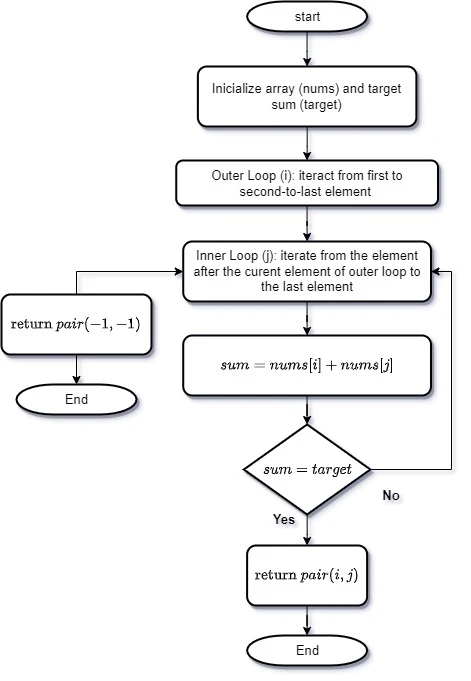 Flowchart 4 - Brute-Force solution for Two-Sum problem
Flowchart 4 enables the creation of a function to solve the two-sum problem in C++20, as can be seen in Code 4 below:
#include <iostream>
#include <vector>
#include <utility>
// Function to find a pair of numbers that add up to the target sum Brute-Force
std::pair<int, int> Values(const std::vector<int>& sequence, int targetSum) {
int n = sequence.size();
// Iterate over all possible pairs
for (int i = 0; i < n - 1; ++i) {
for (int j = i + 1; j < n; ++j) {
// Check if the current pair sums to the target
if (sequence[i] + sequence[j] == targetSum) {
return std::make_pair(sequence[i], sequence[j]); // Pair found
}
}
}
// No pair found
return std::make_pair(-1, -1);
}
int main() {
// Example usage
std::vector<int> sequence = { 8, 10, 2, 9, 7, 5 };
int targetSum = 11;
// Call the function and print the result
std::pair<int, int> result = Values(sequence, targetSum);
if (result.first != -1) {
std::cout << "Pair found: (" << result.first << ", " << result.second << ")" << std::endl;
}
else {
std::cout << "No pair found." << std::endl;
}
return 0;
}
Code 3: Full code of a two-sum using std::vector
The Values function is quite simple, but the use of std::vector and std::pair in Code 4 deserves a closer look. While std::array might offer a slight performance edge, the dynamic nature of std::vector makes it a better fit for interview and competitive programming scenarios where the size of the input data isn’t known in advance. This flexibility is crucial when dealing with data read from external sources like the terminal or text files.
std::pairis a standard template class in C++ used to store a pair of values, which can be of different types. It has been available since C++98 and is defined in the<utility>header. This class is particularly useful for returning two values from a function or for storing two related values together. It has two public member variables,firstandsecond, which store the values. Astd::paircan be initialized using constructors or the helper functionstd::make_pair. The kind reader can create astd::pairdirectly using its constructor (std::pair<int, double> p1(42, 3.14);) or by usingstd::make_pair(auto p2 = std::make_pair(42, 3.14);). It is straightforward to access the membersfirstandseconddirectly (std::cout << "First: " << p1.first << ", Second: " << p1.second << std::endl;). Since C++11, we also havestd::tupleandstd::tie, which extend the functionality ofstd::pairby allowing the grouping of more than two values.std::tuplecan store any number of values of different types, making it more versatile thanstd::pair. Thestd::tiefunction can be used to unpack astd::tupleinto individual variables. Whilestd::pairis simpler and more efficient for just two values,std::tupleprovides greater flexibility for functions needing to return multiple values. For example, astd::tuplecan be created usingstd::make_tuple(auto t = std::make_tuple(1, 2.5, "example");), and its elements can be accessed usingstd::get<index>(t).
The kind reader may have noticed the use of (-1, -1) as sentinel values to indicate that the function did not find any pair. There is a better way to do this. Use the std::optional class as we can see in Code 5:
#include <iostream>
#include <vector>
#include <optional>
#include <utility>
// Function to find a pair of numbers that add up to the target sum
std::optional<std::pair<int, int>> Values(const std::vector<int>& sequence, int targetSum) {
int n = sequence.size();
// Iterate over all possible pairs
for (int i = 0; i < n - 1; ++i) {
for (int j = i + 1; j < n; ++j) {
// Check if the current pair sums to the target
if (sequence[i] + sequence[j] == targetSum) {
return std::make_pair(sequence[i], sequence[j]); // Pair found
}
}
}
// No pair found
return std::nullopt;
}
int main() {
// Example usage
std::vector<int> sequence = {8, 10, 2, 9, 7, 5};
int targetSum = 11;
// Call the function and print the result
if (auto result = Values(sequence, targetSum)) {
std::cout << "Pair found: (" << result->first << ", " << result->second << ")" << std::endl;
} else {
std::cout << "No pair found." << std::endl;
}
return 0;
}
Code 4: Full code of a two-sum using std::vector and std::optional
std::optionalis a feature introduced in C++17 that provides a way to represent optional (or nullable) values. It is a template class that can contain a value or be empty, effectively indicating the presence or absence of a value without resorting to pointers or sentinel values. This makesstd::optionalparticularly useful for functions that may not always return a meaningful result. By usingstd::optional, developers can avoid common pitfalls associated with null pointers and special sentinel values, thereby writing safer and more expressive code.std::optionalis similar to theMaybetype in Haskell, which also represents an optional value that can either beJusta value orNothing. An equivalent in Python is the use ofNoneto represent the absence of a value, often combined with theOptionaltype hint from thetypingmodule to indicate that a function can return either a value of a specified type orNone.
Here is an example of how you can use Optional from the typing module in Python to represent a function that may or may not return a value:
from typing import Optional
def find_min_max(numbers: list[int]) -> Optional[tuple[int, int]]:
if not numbers:
return None
min_val = min(numbers)
max_val = max(numbers)
return min_val, max_val
Code Fragment 12 - Optional implemented in Python
Relying solely on brute-force solutions won’t impress interviewers or win coding competitive programmings. It’s crucial to strive for solutions with lower time complexity whenever possible. While some problems might not have more efficient alternatives, most interview and competitive programming questions are designed to filter out candidates who only know brute-force approaches.
Recursive Approach: Divide and Conquer
The recursive solution leverages a two-pointer approach to efficiently explore the array within a dynamically shrinking window defined by the start and end indices. It operates by progressively dividing the search space into smaller subproblems, each represented by a narrower window, until a base case is reached or the target sum is found. Here’s the refined description, flowchart and code:
Base Cases
-
Empty **Input:** If the array is empty (or if the
startindex is greater than or equal to theendindex), there are no pairs to consider. In this case, we returnstd::nulloptto indicate that no valid pair was found. -
Target Sum Found: If the sum of the elements at the current
startandendindices equals thetargetvalue, we’ve found a matching pair. We return this pair asstd::optional<std::pair<int, int>>to signal success and provide the result.
Recursive Step
-
Explore Leftward: We make a recursive call to the function, incrementing the
startindex by one. This effectively shifts our focus to explore pairs that include the next element to the right of the currentstartposition. -
Explore Rightward (If Necessary): If the recursive call in step 1 doesn’t yield a solution, we make another recursive call, this time decrementing the
endindex by one. This shifts our focus to explore pairs that include the next element to the left of the currentendposition.
This leads us to the illustration of the algorithm in Flowchart 4 and its implementation in C++ Code 5:
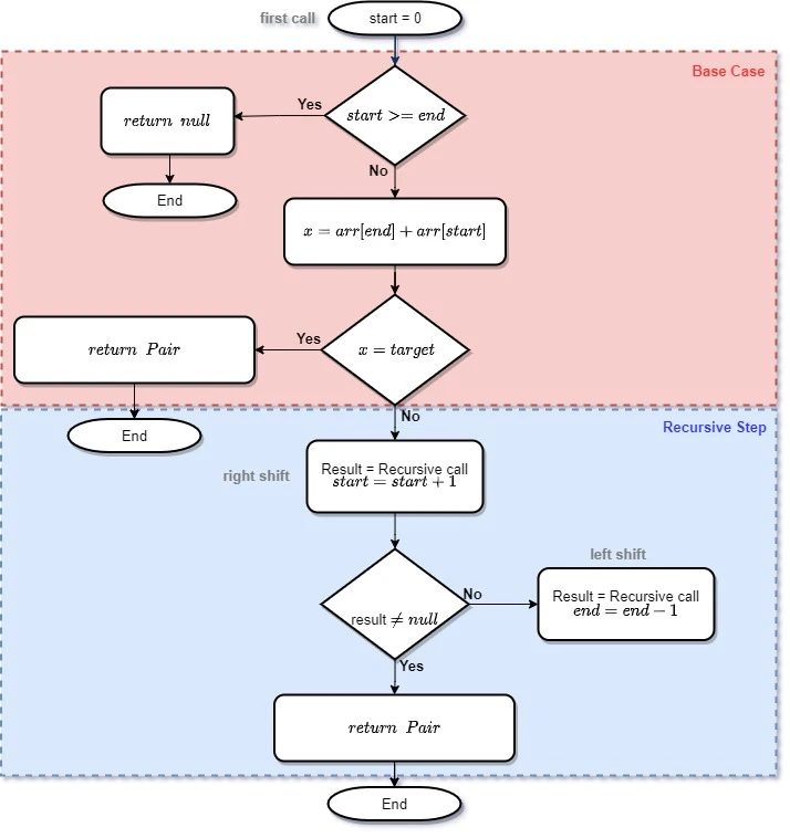 Flowchart 4 - Two-Sum problem recursive solution
#include <vector>
#include <optional>
#include <iostream>
// Recursive function to find a pair of numbers that add up to the target sum
std::optional<std::pair<int, int>> findPairRecursively(const std::vector<int>& arr, int target, int start, int end) {
// Base case: If start index is greater than or equal to end index, no pair is found
if (start >= end) {
return std::nullopt; // Return no value (null optional)
}
// Base case: If the sum of elements at start and end indices equals the target, pair is found
if (arr[start] + arr[end] == target) {
return std::make_optional(std::make_pair(arr[start], arr[end])); // Return the pair
}
// Recursive call: Move the start index forward to check the next element
auto result = findPairRecursively(arr, target, start + 1, end);
if (result) {
return result; // If a pair is found in the recursive call, return it
}
// Recursive call: Move the end index backward to check the previous element
return findPairRecursively(arr, target, start, end - 1);
}
// Function to find a pair of numbers that add up to the target sum
std::optional<std::pair<int, int>> Values(const std::vector<int>& sequence, int targetSum) {
// Call the recursive function with initial indices (0 and size-1)
return findPairRecursively(sequence, targetSum, 0, sequence.size() - 1);
}
int main() {
// Example usage
std::vector<int> sequence = { 8, 10, 2, 9, 7, 5 }; // Input array
int targetSum = 11; // Target sum
// Call the function to find the pair
auto result = Values(sequence, targetSum);
// Print the result
if (result) {
std::cout << "Pair found: (" << result->first << ", " << result->second << ")\n";
} else {
std::cout << "No pair found.\n";
}
return 0;
}
Code 5: Full code of a two-sum using a recursive function
Solution Analysis
The recursion systematically explores all possible pairs in the array by moving the start and end indices in a controlled manner. With each recursive call, the problem is reduced until one of the base cases is reached.
The std::optional<std::pair<int, int>> findPairRecursively(const std::vector<int>& arr, int target, int start, int end) recursive function explores all possible pairs in the array by moving the start and end indices. Let’s analyze its time complexity:
-
Base Case: The base case occurs when
startis greater than or equal toend. In the worst case, this happens after exploring all possible pairs. -
Recursive Calls: For each pair
(start, end), there are two recursive calls:- One that increments the
startindex. - Another that decrements the
endindex.
- One that increments the
Given an array of size n, the total number of pairs to explore is approximately n^2 / 2 (combinatorial pairs). Since each recursive call reduces the problem size by one element, the number of recursive calls can be modeled as a binary tree with a height of n, leading to a total of 2^n calls in the worst case.
Therefore, the recursive function exhibits a time complexity of $O(2^n)$. This exponential complexity arises because each unique pair of indices in the array triggers recursive calls, leading to a rapid increase in computation time as the array size grows. This makes the recursive approach impractical for handling large arrays.
The space complexity, however, is determined by the maximum depth of the recursion stack:
-
Recursion Stack Depth: In the worst-case scenario, the recursive function will delve to a depth of $n$. This happens when each recursive call processes a single element and spawns further recursive calls until it reaches the base case (when a single element remains).
-
Auxiliary Space: Besides the space occupied by the recursion stack, no other substantial amount of memory is utilized.
Consequently, the recursive function’s space complexity is $O(n)$, where $n$ denotes the array size. This linear space complexity results from the recursion stack, which stores information about each function call.
In summary, we have the following characteristics:
- Time Complexity: $O(2^n)$;
- Space Complexity: $O(n)$.
While the recursive approach proves to be highly inefficient in terms of time complexity, rendering it unsuitable for large inputs, it’s crucial to compare its performance with the previously discussed brute-force solutions to gain a comprehensive understanding of its strengths and weaknesses.
The Brute-Force solution to the two-sum problem involves checking all possible pairs in the array to see if any pair meets the desired target value. This approach has a time complexity of $O(n^2)$ because it uses nested loops to iterate over all pairs. The space complexity is $O(1)$ as it does not require additional storage beyond the input array and a few variables.
On the other hand, the recursive solution systematically explores all possible pairs by moving the start and end indices. Although it achieves the same goal, its time complexity is much worse, at $O(2^n)$. This exponential complexity arises because each recursive call generates two more calls, leading to an exponential growth in the number of calls. The space complexity of the recursive solution is $O(n)$, as it requires a recursion stack that can grow up to the depth of the array size.
In summary, while both approaches solve the problem, the Brute-Force solution is significantly more efficient in terms of time complexity ($O(n^2)$ vs. $O(2^n)$), and it also has a lower space complexity ($O(1)$ vs. $O(n)$). However, we are not interested in either of these solutions. The Brute-Force solution is naive and offers no advantage, and the recursive solution is impractical. Thus, we are left with the Dynamic Programming solutions.
Dynamic Programming: memoization
Regardless of the efficiency of the recursive code, the first law of Dynamic Programming says: always start with recursion. Thus, the recursive function will be useful for defining the structure of the code using memoization and tabulation.
Memoization is a technique that involves storing the results of expensive function calls and reusing the cached result when the same inputs occur again. By storing intermediate results, we can avoid redundant calculations, thus optimizing the solution.
In the context of the two-sum problem, memoization can help reduce the number of redundant checks by storing the pairs that have already been evaluated. We’ll use a std::unordered_map to store the pairs of indices we’ve already checked and their sums. This will help us quickly determine if we’ve already computed the sum for a particular pair of indices.
We’ll modify the recursive function to check the memoization map before performing any further calculations. If the pair has already been computed, we’ll use the stored result instead of recalculating. After calculating the sum of a pair, we’ll store the result in the memoization map before returning it. This ensures that future calls with the same pair of indices can be resolved quickly. By using memoization, we aim to reduce the number of redundant calculations, thus improving the efficiency compared to a purely recursive approach.
Memoized Recursive Solution in C++20
The only significant modification in Code 5 is the conversion of the recursive function to Dynamic Programming with memoization. Code 6 presents this updated function.
// Recursive function with memoization to find a pair of numbers that add up to the target sum
std::optional<std::pair<int, int>> findPairRecursivelyMemo(
const std::vector<int>& arr,
int target,
int start,
int end,
std::unordered_map<std::string, std::optional<std::pair<int, int>>>& memo
) {
// Base case: If start index is greater than or equal to end index, no pair is found
if (start >= end) {
return std::nullopt; // Return no value (null optional)
}
// Create a unique key for memoization
std::string key = createKey(start, end);
// Check if the result is already in the memoization map
if (memo.find(key) != memo.end()) {
return memo[key]; // Return the memoized result
}
// Base case: If the sum of elements at start and end indices equals the target, pair is found
if (arr[start] + arr[end] == target) {
auto result = std::make_optional(std::make_pair(arr[start], arr[end]));
memo[key] = result; // Store the result in the memoization map
return result; // Return the pair
}
// Recursive call: Move the start index forward to check the next element
auto result = findPairRecursivelyMemo(arr, target, start + 1, end, memo);
if (result) {
memo[key] = result; // Store the result in the memoization map
return result; // If a pair is found in the recursive call, return it
}
// Recursive call: Move the end index backward to check the previous element
result = findPairRecursivelyMemo(arr, target, start, end - 1, memo);
memo[key] = result; // Store the result in the memoization map
return result; // Return the result
}
Code Fragment 13 - Two-sum using a Memoized function
Complexity Analysis of the Memoized Solution
In the memoized solution, we store the results of the subproblems in a map to avoid redundant calculations. We can analyze the time complexity step-by-step:
-
Base Case Check:
- If the base case is met (when
start >= end), the function returns immediately. This takes constant time, $O(1)$.
- If the base case is met (when
-
Memoization Check:
- Before performing any calculations, the function checks if the result for the current pair of indices (
start,end) is already stored in the memoization map. Accessing the map has an average time complexity of $O(1)$.
- Before performing any calculations, the function checks if the result for the current pair of indices (
-
Recursive Calls:
- The function makes two recursive calls for each pair of indices: one that increments the
startindex and another that decrements theendindex. - In the worst case, without memoization, this would lead to $2^n$ recursive calls due to the binary nature of the recursive calls.
- The function makes two recursive calls for each pair of indices: one that increments the
However, with memoization, each unique pair of indices is computed only once and stored. Given that there are $n(n-1)/2$ unique pairs of indices in an array of size $n$, the memoized function will compute the sum for each pair only once. Thus, the total number of unique computations is limited to the number of pairs, which is $O(n^2)$. Therefore, the time complexity of the memoized solution is O(n^2).
The space complexity of the memoized solution is influenced by two primary factors:
-
Recursion Stack Depth: In the most extreme scenario, the recursion could reach a depth of $n$. This means $n$ function calls would be active simultaneously, each taking up space on the call stack. This contributes $O(n)$ to the space complexity.
-
Memoization Map Size: This map is used to store the results of computations to avoid redundant calculations. The maximum number of unique entries in this map is determined by the number of distinct pairs of indices we can form from a set of $n$ elements. This number is given by the combination formula n^2, which simplifies to $n(n-1)/2$. As each entry in the map takes up constant space, the overall space used by the memoization map is $O(n^2)$.
Combining these two factors, the overall space complexity of the memoized solution is dominated by the larger of the two, which is $O(n^2)$. This leads us to the following conclusions:
- Time Complexity: $O(n^2)$ - The time it takes to process the input grows quadratically with the input size due to the nested loops and memoization overhead.
- Space Complexity: $O(n^2)$ - The amount of memory required for storing memoized results also increases quadratically with the input size because the memoization table grows proportionally to n^2.
By storing the results of subproblems, the memoized solution reduces redundant calculations, achieving a time complexity of $O(n^2)$. The memoization map and recursion stack together contribute to a space complexity of $O(n^2)$. Although it has the same time complexity as the Brute-Force solution, memoization significantly improves efficiency by avoiding redundant calculations, making it more practical for larger arrays.
The Brute-Force solution involves nested loops to check all possible pairs, leading to a time complexity of $O(n^2)$. This solution does not use any additional space apart from a few variables, so its space complexity is $O(1)$. While straightforward, the Brute-Force approach is not efficient for large arrays due to its quadratic time complexity.
The naive recursive solution, on the other hand, explores all possible pairs without any optimization, resulting in an exponential time complexity of $O(2^n)$. The recursion stack can grow up to a depth of $n$, leading to a space complexity of $O(n)$. This approach is highly inefficient for large inputs because it redundantly checks the same pairs multiple times.
At this point we can create a summary table.
| Solution Type | Time Complexity | Space Complexity |
|---|---|---|
| Brute-Force | $O(n^2)$ | $O(1)$ |
| Recursive | $O(2^n)$ | $O(n)$ |
| Memoized | $O(n^2)$ | $O(n^2)$ |
Tabela 3 - Brute-Force, Recursive and Memoized Solutions Complexity Comparison
The situation may seem grim, with the brute-force approach holding the lead as our best solution so far. But don’t lose hope just yet! We have a secret weapon up our sleeves: Dynamic Programming with tabulation.
Dynamic Programming: tabulation
Think of it like this: we’ve been wandering through a maze, trying every path to find the treasure (our solution). The brute-force approach means we’re checking every single path, even ones we’ve already explored. It’s exhausting and time-consuming.
But Dynamic Programming with tabulation is like leaving breadcrumbs along the way. As we explore the maze, we mark the paths we’ve already taken. This way, we avoid wasting time revisiting those paths and focus on new possibilities. It’s a smarter way to navigate the maze and find the treasure faster.
In the context of our problem, tabulation means creating a table to store solutions to smaller subproblems. As we solve larger problems, we can refer to this table to avoid redundant calculations. It’s a clever way to optimize our solution and potentially find the treasure much faster.
So, even though the brute-force approach may seem like the only option right now, don’t give up! Attention! Spoiler Alert! With Dynamic Programming and tabulation, we can explore the maze more efficiently and hopefully find the treasure we’ve been seeking.
C++ code for Two-Sum problem using tabulation
The code is:
#include <iostream>
#include <vector>
#include <unordered_map>
#include <optional>
// Function to find a pair of numbers that add up to the target sum using tabulation
std::optional<std::pair<int, int>> ValuesTabulation(const std::vector<int>& sequence, int targetSum) {
std::unordered_map<int, int> table; // Hash table to store elements and their indices
for (int i = 0; i < sequence.size(); ++i) {
int complement = targetSum - sequence[i];
// Check if the complement exists in the hash table
if (table.find(complement) != table.end()) {
return std::make_optional(std::make_pair(sequence[i], complement)); // Pair found
}
// Store the current element in the hash table
table[sequence[i]] = i;
}
// No pair found
return std::nullopt;
}
int main() {
// Example usage
std::vector<int> sequence = {8, 10, 2, 9, 7, 5}; // Input array
int targetSum = 11; // Target sum
// Call the function to find the pair
auto result = ValuesTabulation(sequence, targetSum);
// Print the result
if (result) {
std::cout << "Pair found: (" << result->first << ", " << result->second << ")\n";
} else {
std::cout << "No pair found.\n";
}
return 0;
}
Code 9: Full code of a two-sum using a tabulated function
The std::optional<std::pair<int, int>> ValuesTabulation(const std::vector<int>& sequence, int targetSum) function uses a hash table (std::unordered_map) to store elements of the array and their indices. For each element in the array, it calculates the complement, which is the difference between the target sum and the current element. It then checks if the complement exists in the hash table. If the complement is found, a pair that sums to the target has been identified and the function returns this pair. If the complement does not exist, the function stores the current element and its index in the hash table and proceeds to the next element.
Complexity Analysis of the Tabulation Function
The std::optional<std::pair<int, int>> ValuesTabulation(const std::vector<int>& sequence, int targetSum) function uses a hash table to efficiently find a pair of numbers that add up to the target sum. The function iterates through each element of the array once, making its time complexity $O(n)$. For each element, it calculates the complement (the difference between the target sum and the current element) and checks if this complement exists in the hash table. Accessing and inserting elements into the hash table both have an average time complexity of $O(1)$, contributing to the overall linear time complexity of the function.
The space complexity of the function is also $O(n)$, as it uses a hash table to store the elements of the array and their indices. The size of the hash table grows linearly with the number of elements in the array, which is why the space complexity is linear.
Comparing this with the other solutions, the Brute-Force solution has a time complexity of $O(n^2)$ because it involves nested loops to check all possible pairs, and its space complexity is $O(1)$ since it uses only a few additional variables. The recursive solution without optimization has an exponential time complexity of $O(2^n)$ due to redundant calculations in exploring all pairs, with a space complexity of $O(n)$ due to the recursion stack. The memoized solution improves upon the naive recursion by storing results of subproblems, achieving a time complexity of $O(n^2)$ and a space complexity of $O(n^2)$ due to the memoization map and recursion stack.
In comparison, the tabulation function is significantly more efficient in terms of both time and space complexity. It leverages the hash table to avoid redundant calculations and provides a linear time solution with linear space usage, making it the most efficient among the four approaches. Wha we can see in the following table.
| Solution Type | Time Complexity | Space Complexity |
|---|---|---|
| Brute-Force | $O(n^2)$ | $O(1)$ |
| Recursive | $O(2^n)$ | $O(n)$ |
| Memoized | $O(n^2)$ | $O(n^2)$ |
| Tabulation | $O(n)$ | $O(n)$ |
Tabela 4 - Brute-Force, Recursive, Memoized and Tabulated Solutions Complexity Comparison
And so, it seems, we have a champion: Dynamic Programming with tabulation! Anyone armed with this technique has a significant advantage when tackling this problem, especially in job interviews where optimization and clever problem-solving are highly valued.
However, let’s be realistic: in the fast-paced world of programming competitive programmings, where every millisecond counts, tabulation might not always be the winner. It can require more memory and setup time compared to other approaches, potentially slowing you down in a race against the clock.
So, while tabulation shines in showcasing your understanding of optimization and problem-solving, it’s important to be strategic in a competitive programming setting. Sometimes, a simpler, faster solution might be the key to victory, even if it’s less elegant.
The bottom line? Mastering Dynamic Programming and tabulation is a valuable asset, but knowing when and where to use it is the mark of a true programming champion. Now, all that’s left is to analyze the execution times.
Execution Time Analysis
I started by testing with the same code we used to test the Fibonacci functions. However, in my initial analysis, I noticed some inconsistencies in the execution times. To address this, I refined our measurement methodology by eliminating lambda functions and directly measuring execution time within the main loop. This removed potential overhead introduced by the lambdas, leading to more reliable results. So, I wrote a new, simpler, and more direct code to test the functions:
#include <iostream>
#include <vector>
#include <unordered_map>
#include <optional>
#include <utility>
#include <chrono>
// Function to measure execution time
template <typename Func, typename... Args>
long long measure_time(Func func, Args&&... args) {
auto start = std::chrono::high_resolution_clock::now();
func(std::forward<Args>(args)...);
auto end = std::chrono::high_resolution_clock::now();
std::chrono::duration<long long, std::nano> duration = end - start;
return duration.count();
}
// Function to calculate average execution time
template <typename Func, typename... Args>
long long average_time(Func func, int iterations, Args&&... args) {
long long total_time = 0;
for (int i = 0; i < iterations; ++i) {
total_time += measure_time(func, std::forward<Args>(args)...);
}
return total_time / iterations;
}
// Brute-Force Solution
std::pair<int, int> ValuesBruteForce(const std::vector<int>& sequence, int targetSum) {
int n = sequence.size();
for (int i = 0; i < n - 1; ++i) {
for (int j = i + 1; j < n; ++j) {
if (sequence[i] + sequence[j] == targetSum) {
return std::make_pair(sequence[i], sequence[j]);
}
}
}
return std::make_pair(-1, -1);
}
// Naive Recursive Solution
std::optional<std::pair<int, int>> findPairRecursively(const std::vector<int>& arr, int target, int start, int end) {
if (start >= end) {
return std::nullopt;
}
if (arr[start] + arr[end] == target) {
return std::make_optional(std::make_pair(arr[start], arr[end]));
}
auto result = findPairRecursively(arr, target, start + 1, end);
if (result) {
return result;
}
return findPairRecursively(arr, target, start, end - 1);
}
std::optional<std::pair<int, int>> ValuesRecursive(const std::vector<int>& sequence, int targetSum) {
return findPairRecursively(sequence, targetSum, 0, sequence.size() - 1);
}
// Memoized Recursive Solution
std::string createKey(int start, int end) {
return std::to_string(start) + "," + std::to_string(end);
}
std::optional<std::pair<int, int>> findPairRecursivelyMemo(
const std::vector<int>& arr, int target, int start, int end,
std::unordered_map<std::string, std::optional<std::pair<int, int>>>& memo) {
if (start >= end) {
return std::nullopt;
}
std::string key = createKey(start, end);
if (memo.find(key) != memo.end()) {
return memo[key];
}
if (arr[start] + arr[end] == target) {
auto result = std::make_optional(std::make_pair(arr[start], arr[end]));
memo[key] = result;
return result;
}
auto result = findPairRecursivelyMemo(arr, target, start + 1, end, memo);
if (result) {
memo[key] = result;
return result;
}
result = findPairRecursivelyMemo(arr, target, start, end - 1, memo);
memo[key] = result;
return result;
}
std::optional<std::pair<int, int>> ValuesMemoized(const std::vector<int>& sequence, int targetSum) {
std::unordered_map<std::string, std::optional<std::pair<int, int>>> memo;
return findPairRecursivelyMemo(sequence, targetSum, 0, sequence.size() - 1, memo);
}
// Tabulation Solution
std::optional<std::pair<int, int>> ValuesTabulation(const std::vector<int>& sequence, int targetSum) {
std::unordered_map<int, int> table;
for (int i = 0; i < sequence.size(); ++i) {
int complement = targetSum - sequence[i];
if (table.find(complement) != table.end()) {
return std::make_optional(std::make_pair(sequence[i], complement));
}
table[sequence[i]] = i;
}
return std::nullopt;
}
int main() {
std::vector<int> sequence = {8, 10, 2, 9, 7, 5};; // 40 numbers
int targetSum = 11;
int iterations = 1000;
std::cout << "-----------------------------------\n";
std::cout << "Calculating Two-Sum (" << targetSum << ")\n";
// Measure average execution time for Brute-Force Solution
auto bruteForceTime = average_time([](const std::vector<int>& seq, int target) {
ValuesBruteForce(seq, target);
}, iterations, sequence, targetSum);
std::cout << "Average time for Brute-Force: " << bruteForceTime << " ns\n";
// Measure average execution time for Naive Recursive Solution
auto recursiveTime = average_time([](const std::vector<int>& seq, int target) {
ValuesRecursive(seq, target);
}, iterations, sequence, targetSum);
std::cout << "Average time for Recursive: " << recursiveTime << " ns\n";
// Measure average execution time for Memoized Recursive Solution
auto memoizedTime = average_time([](const std::vector<int>& seq, int target) {
ValuesMemoized(seq, target);
}, iterations, sequence, targetSum);
std::cout << "Average time for Memoized: " << memoizedTime << " ns\n";
// Measure average execution time for Tabulation Solution
auto tabulationTime = average_time([](const std::vector<int>& seq, int target) {
ValuesTabulation(seq, target);
}, iterations, sequence, targetSum);
std::cout << "Average time for Tabulation: " << tabulationTime << " ns\n";
std::cout << "-----------------------------------\n";
return 0;
}
Code 10: Code for execution time test of all functions we create to Two-Sum problem.
I simply replicated the functions from the previous code snippets, without any optimization, precisely because our current objective is to solely examine the execution times. Running the new code, we have the following Output:
-----------------------------------
Calculating Two-Sum (18)
Average time for Brute-Force: 217 ns
Average time for Recursive: 415 ns
Average time for Memoized: 41758 ns
Average time for Tabulation: 15144 ns
-----------------------------------
Output 4: Execution time of Two-Sum solutions.
As we’ve seen, when dealing with a small amount of input data, the brute-force approach surprisingly outshines even more complex algorithms. This might seem counterintuitive, but it’s all about the hidden costs of memory management.
When we use sophisticated data structures like std::string and std::unordered_map, we pay a price in terms of computational overhead. Allocating and deallocating memory on the heap for these structures takes time and resources. This overhead becomes especially noticeable when dealing with small datasets, where the time spent managing memory can easily overshadow the actual computation involved. On the other hand, the brute-force method often relies on simple data types and avoids dynamic memory allocation, resulting in a faster and more efficient solution for smaller inputs.
The Dynamic Memory Bottleneck
There are some well-known bottlenecks that can explain why a code with lower complexity runs much slower in a particular environment.
Hash Table Overhead: Both memoized and tabulation solutions rely on std::unordered_map, which inherently involves dynamic memory allocation. Operations like insertions and lookups, while powerful, come with a cost due to memory management overhead. This is typically slower than accessing elements in a simple array.
Recursion’s Toll: The naive recursive and memoized solutions utilize deep recursion, leading to a considerable overhead from managing the recursion stack. Each recursive call adds a new frame to the stack, requiring additional memory operations that accumulate over time.
Memoization’s Complexity: While memoization optimizes by storing intermediate results, it also introduces complexity through the use of std::unordered_map. Each new pair calculated requires storage in the hash table, involving dynamic allocations and hash computations, adding to the overall time complexity.
Cache Friendliness: Dynamic memory allocations often lead to suboptimal cache utilization. In contrast, the Brute-Force and tabulation solutions likely benefit from better cache locality due to their predominant use of array accesses. Accessing contiguous memory locations (as in arrays) generally results in faster execution due to improved cache hit rates.
Function Call Overhead: The overhead from frequent function calls, including those made through lambda functions, can accumulate, particularly in performance-critical code.
By understanding and mitigating these bottlenecks, we can better optimize our code and achieve the expected performance improvements.
In essence, the dynamic nature of memory operations associated with hash tables and recursion significantly affects execution times. These operations are generally slower than accessing static memory structures like arrays. The deep recursion in the memoized and naive recursive approaches exacerbates this issue, as the growing recursion stack necessitates increased memory management.
The memoized solution, while clever, bears the brunt of both issues – extensive recursion and frequent hash table operations. This combination leads to higher execution times compared to the Brute-Force and tabulation approaches, which primarily rely on array accesses and enjoy the benefits of better cache performance and reduced memory management overhead.
In conclusion, the observed differences in execution times can be attributed to the distinct memory access patterns and associated overheads inherent in each approach. Understanding these nuances is crucial for making informed decisions when optimizing code for performance.
We will always have C
As we delve into Dynamic Programming with C++, our focus is on techniques that shine in interviews and coding competitive programmings. Since competitive coding often favors slick C-style code, we’ll zero in on a tabulation solution for this problem. Tabulation, as we know, is usually the most efficient approach. To show you what I mean, check out the int* ValuesTabulationCStyle(const int* sequence, int length, int targetSum) function in Code Fragment 12.
int* ValuesTabulationCStyle(const int* sequence, int length, int targetSum) {
const int MAX_VAL = 1000; // Assuming the values in the sequence are less than 1000
static int result[2] = { -1, -1 }; // Static array to return the result
int table[MAX_VAL];
memset(table, -1, sizeof(table));
for (int i = 0; i < length; ++i) {
int complement = targetSum - sequence[i];
if (complement >= 0 && table[complement] != -1) {
result[0] = sequence[i];
result[1] = complement;
return result;
}
table[sequence[i]] = i;
}
return result;
}
Code Fragment 14 - Two-sum with C-Style code, using a Memoized Function
The C-style function is as straightforward as it gets, and as far as I can tell, it’s equivalent to the C++ tabulation function. Perhaps the only thing worth noting is the use of the memset function.
The
memsetfunction in C and C++ is your go-to tool for filling a block of memory with a specific value. You’ll usually find it defined in the<cstring>header. It takes a pointer to the memory block you want to fill (ptr), the value you want to set (converted to anunsigned char), and the number of bytes you want to set. In our code,memset(table, -1, sizeof(table)); does exactly that—it fills the entire table array with the value $-1$, which is a handy way to mark those spots as empty or unused. Why usememsetinstead ofmallocoralloc? Well,memsetis all about initializing memory that’s already been allocated.mallocandallocare for allocating new memory. If you need to do both, C++ has you covered with thenewoperator, which can allocate and initialize in one step. So,memsetis the memory magician for resetting or initializing arrays and structures, whilemalloc,alloc, andcallochandle the memory allocation part of the job.
The use of menset bring us to analise the function complexity.
Two-Sum C-Style Tabulation Function Complexity
The function ValuesTabulationCStyle uses memset to initialize the table array. The complexity of the function can be divided into two parts:
-
Initialization with
memset:memset(table, -1, sizeof(table));The memset function initializes each byte of the array. Since the size of the array is constant (
MAX_VAL), the complexity of this operation is $O(1)$ in terms of asymptotic complexity, although it has a constant cost depending on the array size.for (int i = 0; i < length; ++i) { int complement = targetSum - sequence[i]; if (complement >= 0 && table[complement] != -1) { result[0] = sequence[i]; result[1] = complement; return result; } table[sequence[i]] = i; } -
The Main Loop
The main loop iterates over each element of the input array sequence. Therefore, the complexity of this part is $O(n)$, where n is the length of the sequence array.
Combining all the pieces, the function’s overall complexity is still $O(n)$. Even though initializing the array with memset takes $O(1)$ time, it doesn’t change the fact that we have to loop through each element in the input array, which takes $O(n)$ time.
Looking back at our original C++ function using std::unordered_map, we also had O(1) complexity for the map initialization and O(n) for the main loop. So, while using memset for our C-style array feels different, it doesn’t change the big picture – both approaches end up with linear complexity.
The key takeaway here is that while using memset might feel like a win for initialization time, it doesn’t change the overall complexity when you consider the whole function. This leaves us with the task of running the code and analyzing the execution times, as shown in Output 5.
-----------------------------------
Calculating Two-Sum (11)
Average time for Brute-Force: 318 ns
Average time for Recursive: 626 ns
Average time for Memoized: 39078 ns
Average time for Tabulation: 5882 ns
Average time for Tabulation C-Style: 189 ns
-----------------------------------
Output 5: Execution time of Two-Sum solutions, including C-Style Arrays.
Analyzing Output 5, it’s clear that the C-style solution is, for all intents and purposes, twice as fast as the C++ tabulation solution. However, there are a few caveats: the C++ code was written to showcase the language’s flexibility, not to optimize for performance. On the other hand, the C-style function was designed for simplicity. Often, simplicity equates to speed, and this is something to maximize when creating a function with linear complexity. Now, we need to compare the C solution with C++ code that prioritizes high performance over flexibility in writing.
High Performance C++
Code Fragment 15 was rewritten by stripping away all the complex data structures we were previously using. The main() function remains largely unchanged, so it’s been omitted here. I’ve also removed the functions used for measuring and printing execution times.
// Brute-Force Solution
std::array<int, 2> ValuesBruteForce(const std::vector<int>& sequence, int targetSum) {
int n = sequence.size();
for (int i = 0; i < n - 1; ++i) {
for (int j = i + 1; j < n; ++j) {
if (sequence[i] + sequence[j] == targetSum) {
return { sequence[i], sequence[j] };
}
}
}
return { -1, -1 };
}
// Naive Recursive Solution
std::array<int, 2> findPairRecursively(const std::vector<int>& arr, int target, int start, int end) {
if (start >= end) {
return { -1, -1 };
}
if (arr[start] + arr[end] == target) {
return { arr[start], arr[end] };
}
std::array<int, 2> result = findPairRecursively(arr, target, start + 1, end);
if (result[0] != -1) {
return result;
}
return findPairRecursively(arr, target, start, end - 1);
}
std::array<int, 2> ValuesRecursive(const std::vector<int>& sequence, int targetSum) {
return findPairRecursively(sequence, targetSum, 0, sequence.size() - 1);
}
// Memoized Recursive Solution
std::array<int, 2> findPairRecursivelyMemo(
const std::vector<int>& arr, int target, int start, int end,
std::array<std::array<int, 2>, 1000>& memo) {
if (start >= end) {
return { -1, -1 };
}
if (memo[start][end][0] != -1) {
return memo[start][end];
}
if (arr[start] + arr[end] == target) {
memo[start][end] = { arr[start], arr[end] };
return { arr[start], arr[end] };
}
std::array<int, 2> result = findPairRecursivelyMemo(arr, target, start + 1, end, memo);
if (result[0] != -1) {
memo[start][end] = result;
return result;
}
result = findPairRecursivelyMemo(arr, target, start, end - 1, memo);
memo[start][end] = result;
return result;
}
std::array<int, 2> ValuesMemoized(const std::vector<int>& sequence, int targetSum) {
std::array<std::array<int, 2>, 1000> memo;
for (auto& row : memo) {
row = { -1, -1 };
}
return findPairRecursivelyMemo(sequence, targetSum, 0, sequence.size() - 1, memo);
}
// Tabulation Solution using C-style arrays
std::array<int, 2> ValuesTabulationCStyle(const int* sequence, int length, int targetSum) {
const int MAX_VAL = 1000; // Assuming the values in the sequence are less than 1000
std::array<int, 2> result = { -1, -1 }; // Static array to return the result
int table[MAX_VAL];
memset(table, -1, sizeof(table));
for (int i = 0; i < length; ++i) {
int complement = targetSum - sequence[i];
if (complement >= 0 && table[complement] != -1) {
result[0] = sequence[i];
result[1] = complement;
return result;
}
table[sequence[i]] = i;
}
return result;
}
Code Fragment 15 - All Two-sum functions including a pure std::array tabulated function
Running this modified code, we get the following Output:
-----------------------------------
Calculating Two-Sum (11)
Average time for Brute-Force: 157 ns
Average time for Recursive: 652 ns
Average time for Memoized: 39514 ns
Average time for Tabulation: 5884 ns
Average time for Tabulation C-Style: 149 ns
-----------------------------------
Output 6: Execution time of All Two-Sum solutions including C-style Tabulation.
Let’s break down the results for calculating the Two-Sum problem, keeping in mind that the fastest solutions have a linear time complexity, O(n):
- Brute-Force: Blazing fast at 157 ns on average. This is our baseline, but remember, Brute-Force doesn’t always scale well for larger problems.
- Recursive: A bit slower at 652 ns. Recursion can be elegant, but it can also lead to overhead.
- Memoized: This one’s the outlier at 39514 ns. Memoization can be a powerful optimization, but it looks like the overhead is outweighing the benefits in this case.
- Tabulation: A respectable 5884 ns. Tabulation is a solid Dynamic Programming technique, and it shows here.
- Tabulation C-Style: A close winner at 149 ns! This stripped-down, C-style implementation of tabulation is just a hair behind Brute-Force in terms of speed.
The C++ and C versions of our tabulation function are practically neck and neck in terms of speed for a few key reasons:
-
Shared Simplicity: Both versions use plain old arrays (
std::arrayin C++, C-style arrays in C) to store data. This means memory access is super efficient in both cases. -
Speedy Setup: We use
memsetto initialize the array in both versions. This is a highly optimized operation, so the initialization step is lightning fast in both languages. -
Compiler Magic: Modern C++ compilers are incredibly smart. They can often optimize the code using
std::arrayto be just as fast, or even faster, than hand-written C code. -
No Frills: Both functions have a straightforward design without any fancy branching or extra layers. The operations within the loops are simple and take the same amount of time every time, minimizing any overhead.
-
Compiler Boost: Compilers like GCC and Clang have a whole bag of tricks to make code run faster, like loop unrolling and smart prediction. These tricks work equally well for both C and C++ code, especially when we’re using basic data structures and simple algorithms.
Thanks to all this, the C++ version of our function, using std::array, runs just as fast as its C counterpart.
And this is how C++ code should be for competitive programmings. However, not for interviews. In interviews, unless high performance is specifically requested, what they’re looking for is your mastery of the language and the most efficient algorithms. So, an O(n) solution using the appropriate data structures will give you a better chance of success.
Exercises: Variations of the Two Sum
There are few interesting variations of Two-Sum problem:
- The array can contain both positive and negative integers.
- Each input would have exactly one solution, and you may not use the same element twice.
- Each input can have multiple solutions, and the same element cannot be used twice in a pair.
- The function should return all pairs that sum to the target value.
Try to solve these variations. Take as much time as you need; I will wait.
The Dynamic Programming Classic Problems
From now on, we will explore 10 classic Dynamic Programming problems. For each one, we will delve into Brute-Force techniques, recursion, memoization, tabulation, and finally the most popular solution for each, even if it is not among the techniques we have chosen. The problems we will address are listed in the table below[^1].
| Name | Description/Example |
|---|---|
| Counting all possible paths in a matrix | Given $N$ and $M$, count all possible distinct paths from $(1,1)$ to $(N, M)$, where each step is either from $(i,j)$ to $(i+1,j)$ or $(i,j+1)$. |
| Subset Sum | Given $N$ integers and $T$, determine whether there exists a subset of the given set whose elements sum up to $T$. |
| Longest Increasing Subsequence | You are given an array containing $N$ integers. Your task is to determine the LCS in the array, i.e., LCS where every element is larger than the previous one. |
| Rod Cutting | Given a rod of length $n$ units, Given an integer array cuts where cuts[i] denotes a position you should perform a cut at. The cost of one cut is the length of the rod to be cut. What is the minimum total cost of the cuts. |
| Longest Common Subsequence | You are given strings $s$ and $t$. Find the length of the longest string that is a subsequence of both $s$ and $t$. |
| Longest Palindromic Subsequence | Finding the Longest Palindromic Subsequence (LPS) of a given string. |
| Edit Distance | The edit distance between two strings is the minimum number of operations required to transform one string into the other. Operations are [“Add”, “Remove”, “Replace”]. |
| Coin Change Problem | Given an array of coin denominations and a target amount, find the minimum number of coins needed to make up that amount. |
| 0-1 knapsack | Given $W$, $N$, and $N$ items with weights $w_i$ and values $v_i$, what is the maximum $\sum_{i=1}^{k} v_i$ for each subset of items of size $k$ ($1 \le k \le N$) while ensuring $\sum_{i=1}^{k} w_i \le W$? |
| Longest Path in a Directed Acyclic Graph (DAG) | Finding the longest path in Directed Acyclic Graph (DAG). |
| Traveling Salesman Problem (TSP) | Given a list of cities and the distances between each pair of cities, find the shortest possible route that visits each city exactly once and returns to the origin city. |
| Matrix Chain Multiplication | Given a sequence of matrices, find the most efficient way to multiply these matrices together. The problem is not actually to perform the multiplications, but merely to decide in which order to perform the multiplications. |
Tabela 5 - The Dynamic Programming we’ll study and solve.
Stop for a moment, perhaps have a soda or a good wine. Rest a bit, then gather your courage, arm yourself with patience, and continue. Practice makes perfect.
This will continue!!!
Problem 1 Statement: Counting All Possible Paths in a Matrix
Given two integers $m$ and $n$, representing the dimensions of a matrix, count all possible distinct paths from the top-left corner $(0,0)$ to the bottom-right corner $(m-1,n-1)$. Each step can either be to the right or down.
Input:
- Two integers $m$ and $n$ where $1 \leq m, n \leq 100$.
#*Output:
- An integer representing the number of distinct paths from $(0,0)$ to $(m-1,n-1)$.
Example:
Input: 3 3
Output: 6
Constraints:
- You can only move to the right or down in each step.
Analysis:
Let’s delve deeper into the “unique paths” problem. Picture a matrix as a grid, where you start at the top-left corner $(0, 0)$ and your goal is to reach the bottom-right corner $(m-1, n-1)$. The twist? You’re only allowed to move down or right. The challenge is to figure out how many distinct paths you can take to get from start to finish.
This problem so intriguing because it blends the elegance of combinatorics (the study of counting) with the power of Dynamic Programming (a clever problem-solving technique). The solution involves combinations, a fundamental concept in combinatorics. Moreover, it’s a classic example of how Dynamic Programming can streamline a seemingly complex problem.
The applications of this type of problem extend beyond theoretical interest. They can be found in practical scenarios like robot navigation in a grid environment, calculating probabilities in games with grid-like movements, and analyzing maze-like structures. Understanding this problem provides valuable insights into a range of fields, from mathematics to robotics and beyond.
Now, let’s bring in some combinatorics! To journey from the starting point $(0, 0)$ to the destination $(m-1, n-1)$, you’ll need a total of $(m - 1) + (n - 1)$ moves. That’s a mix of downward and rightward steps.
The exciting part is figuring out how many ways we can arrange those moves. Imagine choosing $(m - 1)$ moves to go down and $(n - 1)$ moves to go right, out of a total of $(m + n - 2)$ moves. This can be calculated using the following formula:
\[C(m + n - 2, m - 1) = \frac{(m + n - 2)!}{(m - 1)! * (n - 1)!}\]For our 3x3 matrix example $(m = 3, n = 3)$, the calculation is:
\[C(3 + 3 - 2, 3 - 1) = \frac{4!}{(2! * 2!)} = 6\]This tells us there are $6$ distinct paths to reach the bottom-right corner. Let’s also visualize this using Dynamic Programming:
Filling the Matrix with Dynamic Programming:
-
Initialize: Start with a $dp$ matrix where $dp[0][0] = 1$ (one way to be at the start).
dp = \begin{bmatrix} 1 & 0 & 0
0 & 0 & 0
0 & 0 & 0 \end{bmatrix} -
Fill First Row and Column: There’s only one way to reach each cell in the first row and column (either from the left or above).
dp = \begin{bmatrix} 1 & 1 & 1
1 & 0 & 0
1 & 0 & 0 \end{bmatrix} -
Fill Remaining Cells: For the rest, the number of paths to a cell is the sum of paths to the cell above and the cell to the left: $dp[i][j] = dp[i-1][j] + dp[i][j-1]$
dp = \begin{bmatrix} 1 & 1 & 1
1 & 2 & 3
1 & 3 & 6 \end{bmatrix}
The bottom-right corner, $dp[2][2]$, holds our answer: $6$ unique paths.
Bear with me, dear reader, as I temporarily diverge from our exploration of Dynamic Programming. Before delving deeper, it’s essential to examine how we might solve this problem using a Brute-Force approach.
Using Brute-Force
To tackle the unique paths problem with a Brute-Force approach, we can use an iterative solution and a stack in C++20. The stack will keep track of our current position in the matrix and the number of paths that led us there. Here’s a breakdown of how it works:
-
We’ll define a structure called
Positionto store the current coordinates $(i, j)$ and the count of paths leading to that position. -
We’ll start by pushing the initial position $(0, 0)$ onto the stack, along with a path count of $1$ (since there’s one way to reach the starting point).
-
While the stack isn’t empty:
- Pop the top position from the stack.
- If we’ve reached the bottom-right corner $(m-1, n-1)$, increment the total path count.
- If moving right is possible (within the matrix bounds), push the new position (with the same path count) onto the stack.
- If moving down is possible, do the same.
-
When the stack is empty, the total path count will be the answer we seek – the total number of unique paths from $(0, 0)$ to $(m-1, n-1)$.
Code Fragment 16 demonstrates how to implement this algorithm in C++.
#include <iostream>
#include <stack>
#include <chrono>
//.....
// Structure to represent a position in the matrix
struct Position {
int i, j;
int pathCount;
};
// Function to count paths using Brute-Force
int countPaths(int m, int n) {
std::stack<Position> stk;
stk.push({ 0, 0, 1 });
int totalPaths = 0;
while (!stk.empty()) {
Position pos = stk.top();
stk.pop();
int i = pos.i, j = pos.j, pathCount = pos.pathCount;
// If we reach the bottom-right corner, add to total paths
if (i == m - 1 && j == n - 1) {
totalPaths += pathCount;
continue;
}
// Move right if within bounds
if (j + 1 < n) {
stk.push({ i, j + 1, pathCount });
}
// Move down if within bounds
if (i + 1 < m) {
stk.push({ i + 1, j, pathCount });
}
}
return totalPaths;
}
Code Fragment 16 - Count all paths function using Brute-Force.
Let’s start looking at std::stack data structure:
In C++20, the
std::stackis a part of the Standard Template Library (STL) and is used to implement a stack data structure, which follows the Last-In-First-Out (LIFO) principle. Astd::stackis a container adapter that provides a stack interface, designed to operate in a LIFO context. Elements are added to and removed from the top of the stack. The syntax for creating a stack isstd::stack<T> stack_name;whereTis the type of elements contained in the stack. To create a stack, you can use constructors such asstd::stack<int> s1;for the default constructor orstd::stack<int> s2(some_container);to construct with a container. To add an element to the top of the stack, use thepushfunction:stack_name.push(value);. To remove the element at the top of the stack, use thepopfunction:stack_name.pop();. To return a reference to the top element of the stack, useT& top_element = stack_name.top();. To check whether the stack is empty, usebool is_empty = stack_name.empty();. Finally, to return the number of elements in the stack, usestd::size_t stack_size = stack_name.size();. Thestd::stackclass is a simple and effective way to manage a stack of elements, ensuring efficient access and modification of the last inserted element.
In the context of our code for counting paths in a matrix using a stack, the line stk.push({ 0, 0, 1 }); is used to initialize the stack with the starting position of the matrix traversal. The stk is a std::stack of Position structures. The Position structure is defined as follows:
struct Position {
int i, j;
int pathCount;
};
The Position structure has three members: i and j, which represent the current coordinates in the matrix, and pathCount, which represents the number of paths that lead to this position.
The line stk.push({ 0, 0, 1 }); serves a specific purpose in our algorithm:
- It creates a
Positionobject with the initializer list{ 0, 0, 1 }, settingi = 0,j = 0, andpathCount = 1. - It then pushes this
Positionobject onto the stack using thepushfunction ofstd::stack.
In simpler terms, this line of code initializes the stack with the starting position of the matrix traversal, which is the top-left corner of the matrix at coordinates $(0, 0)$. It also sets the initial path count to $1$, indicating that there is one path starting from this position. From here, the algorithm will explore all possible paths from the top-left corner.
The Brute-Force solution for counting paths in a matrix involves exploring all possible paths from the top-left corner to the bottom-right corner. Each path consists of a series of moves either to the right or down. The algorithm uses a stack to simulate the recursive exploration of these paths.
To analyze the time complexity, consider that the function must explore each possible combination of moves in the matrix. For a matrix of size $m \times n$, there are a total of $m + n - 2$ moves required to reach the bottom-right corner from the top-left corner. Out of these moves, $m - 1$ must be down moves and $n - 1$ must be right moves. The total number of distinct paths is given by the binomial coefficient $C(m+n-2, m-1)$, which represents the number of ways to choose $m-1$ moves out of $m+n-2$.
The time complexity of the Brute-Force approach is exponential in nature because it explores every possible path. Specifically, the time complexity is $O(2^{m+n})$ since each step involves a choice between moving right or moving down, leading to $2^{m+n}$ possible combinations of moves in the worst case. This exponential growth makes the Brute-Force approach infeasible for large matrices, as the number of paths grows very quickly with increasing $m$ and $n$.
The space complexity is also significant because the algorithm uses a stack to store the state of each position it explores. In the worst case, the depth of the stack can be as large as the total number of moves, which is $m + n - 2$. Thus, the space complexity is $O(m+n)$, primarily due to the stack’s storage requirements.
In summary, the Brute-Force solution has an exponential time complexity $O(2^{m+n})$ and a linear space complexity $O(m+n)$, making it suitable only for small matrices where the number of possible paths is manageable.
My gut feeling tells me this complexity is very, very bad. We’ll definitely find better complexities as we explore Dynamic Programming solutions. Either way, we need to measure the runtime. Running the function int countPaths(int m, int n) within the same structure we created earlier to measure execution time, we will have:
-----------------------------------
Calculating Paths in a 3x3 matrix
Average time for Brute-Force: 10865 ns
-----------------------------------
Output 7: Execution time of Counting all paths problem using Brute-Force.
Finally, I won’t be presenting the code done with pure recursion. As we’ve seen, recursion is very elegant and can score points in interviews. However, the memoization solution will include recursion, so if you use memoization and recursion in the same solution, you’ll ace the interview.
Using Memoization
Code Fragment 17 shows the functions I created to apply memoization. There are two functions: the int countPathsMemoizationWrapper(int m, int n) function used to initialize the dp data structure and call the recursive function int countPathsMemoization(int m, int n, std::vector<std::vector<int>>& dp). I used std::vector already anticipating that we won’t know the size of the matrix beforehand.
// Function to count paths using Dynamic Programming with memoization
int countPathsMemoization(int m, int n, std::vector<std::vector<int>>& dp) {
if (m == 1 || n == 1) return 1; // Base case
if (dp[m - 1][n - 1] != -1) return dp[m - 1][n - 1]; // Return memoized result
dp[m - 1][n - 1] = countPathsMemoization(m - 1, n, dp) + countPathsMemoization(m, n - 1, dp); // Memoize result
return dp[m - 1][n - 1];
}
int countPathsMemoizationWrapper(int m, int n) {
std::vector<std::vector<int>> dp(m, std::vector<int>(n, -1));
return countPathsMemoization(m, n, dp);
}
Code Fragment 17 - Count all paths function using Memoization.
The function int countPathsMemoization(int m, int n, std::vector<std::vector<int>>& dp) counts all possible paths in an $m \times n$ matrix using Dynamic Programming with memoization. The dp matrix serves as a cache, storing and reusing intermediate results to avoid redundant calculations.
Upon invocation, the function first checks if the current position is in the first row (m == 1) or first column (n == 1). If so, it returns $1$, as there is only one way to reach such cells. Next, it checks the dp[m-1][n-1] cell. If the value is not $-1$ (the initial value indicating “not yet calculated”), it signifies that the result for this position has already been memoized and is immediately returned.
Otherwise, the function recursively calculates the number of paths from the cell above (m-1, n) and the cell to the left (m, n-1). The sum of these values is then stored in dp[m-1][n-1] before being returned.
Utilizing std::vector<std::vector<int>> for dp ensures efficient storage of intermediate results, significantly reducing the number of recursive calls required compared to a purely recursive approach. This memoized version substantially improves the function’s performance, especially for larger matrices.
The countPathsMemoization function exemplifies memoization rather than tabulation due to its top-down recursive approach, where results are stored on-the-fly. Memoization involves recursive function calls that cache subproblem results upon their first encounter, ensuring each subproblem is solved only once and reused when needed.
Conversely, tabulation employs a bottom-up approach, utilizing an iterative method to systematically fill a table (or array) with subproblem solutions. This typically begins with the smallest subproblems, iteratively combining results to solve larger ones until the final solution is obtained.
In countPathsMemoization, the function checks if the result for a specific cell is already computed and stored in the dp matrix. If not, it recursively computes the result by combining the results of smaller subproblems and then stores it in the dp matrix. This process continues until all necessary subproblems are solved, a characteristic of memoization.
The dp matrix is utilized to store intermediate results, preventing redundant calculations. Each cell within dp corresponds to a subproblem, representing the number of paths to that cell from the origin. Recursive calls compute the number of paths to a given cell by summing the paths from the cell above and the cell to the left.
The function boasts a time complexity of $O(m \times n)$. This is because each cell in the dp matrix is computed only once, with each computation requiring constant time. Thus, the total operations are proportional to the number of cells in the matrix, namely $m \times n$.
Similarly, the space complexity is $O(m \times n)$ due to the dp matrix, which stores the number of paths for each cell. The matrix necessitates $m \times n$ space to accommodate these intermediate results.
In essence, the Dynamic Programming approach with memoization transforms the exponential time complexity of the naive Brute-Force solution into a linear complexity with respect to the matrix size. Consequently, this solution proves far more efficient and viable for larger matrices.
Finally, we need to run this code and compare it to the Brute-Force version.
-----------------------------------
Calculating Paths in a 3x3 matrix
Average time for Brute-Force: 12494 ns
Average time for Memoization: 4685 ns
-----------------------------------
Output 9: Comparison between Brute-Force, Memoization and Tabulation functions.
I ran it dozens of times and, most of the time, the memoized function was twice as fast as the Brute-Force function, and sometimes it was three times faster. Now we need to look at the Dynamic Programming solution using tabulation.
Using Tabulation
Like I did before, the Code Fragment 18 shows the function I created to apply tabulation. The function int countPathsTabulation(int m, int n) uses Dynamic Programming with tabulation to count all possible paths in an $m \times n$ matrix.
// Function to count paths using Dynamic Programming with tabulation
int countPathsTabulation(int m, int n) {
std::vector<std::vector<int>> dp(m, std::vector<int>(n, 0));
for (int i = 0; i < m; ++i) {
for (int j = 0; j < n; ++j) {
if (i == 0 || j == 0) {
dp[i][j] = 1;
} else {
dp[i][j] = dp[i - 1][j] + dp[i][j - 1];
}
}
}
return dp[m - 1][n - 1];
}
Code Fragment 18 - Count all paths function using Tabulation.
The function int countPathsTabulation(int m, int n) counts all possible paths in an $m \times n$ matrix using Dynamic Programming with tabulation. The dp matrix is used to store the number of paths to each cell in a bottom-up manner, ensuring that each subproblem is solved iteratively. Each subproblem represents the number of distinct paths to a cell $(i, j)$ from the top-left corner $(0, 0)$.
The function initializes a dp matrix of size $m \times n$ with all values set to $0$. It then iterates over each cell in the matrix. If a cell is in the first row or first column, it sets the value to $1$ because there is only one way to reach these cells (either all the way to the right or all the way down). For other cells, it calculates the number of paths by summing the values from the cell above (dp[i - 1][j]) and the cell to the left (dp[i][j - 1]). This sum is then stored in dp[i][j].
Using std::array<std::array<int, MAX_SIZE>, MAX_SIZE> for the dp matrix ensures efficient storage and retrieval of intermediate results. This tabulated approach systematically fills the dp matrix from the smallest subproblems up to the final solution, avoiding the overhead of recursive function calls and providing a clear and straightforward iterative solution.
The time complexity of this function is $O(m \times n)$. Each cell in the dp matrix is computed once, and each computation takes constant time, making the total number of operations proportional to the number of cells in the matrix. Similarly, the space complexity is $O(m \times n)$ due to the dp matrix, which requires $m \times n$ space to store the number of paths for each cell.
This Dynamic Programming approach with tabulation significantly improves performance compared to the naive Brute-Force solution. By transforming the problem into a series of iterative steps, it provides an efficient and scalable solution for counting paths in larger matrices.
Here’s something interesting, dear reader. While using std::vector initially yielded similar execution times to the memoization function, switching to std::array resulted in a dramatic improvement. Not only did it significantly reduce memory usage, but it also made the function up to 4 times faster!
After running additional tests, the tabulation function averaged $3$ times faster execution than the original. However, there’s a caveat: using std::array necessitates knowing the input size beforehand, which might not always be practical in real-world scenarios. Finally we can take a look in this function execution time:
-----------------------------------
Calculating Paths in a 3x3 matrix
Average time for Brute-Force: 10453 ns
Average time for Memoization: 5348 ns
Average time for Tabulation: 1838 ns
-----------------------------------
The key takeaway is this: both memoization and tabulation solutions share the same time complexity. Therefore, in an interview setting, the choice between them boils down to personal preference. But if performance is paramount, tabulation (especially with std::array if the input size is known) is the way to go. Of course, now it’s up to the diligent reader to test all the functions we’ve developed to solve problem “Counting All Possible Paths in a Matrix” with std::array. Performance has its quirks, and since there are many factors outside the programmer’s control involved in execution, we always need to test in the an environment just like the production environment.
Problem 2 Statement: Subset Sum
Given $N$ integers and $T$, determine whether there exists a subset of the given set whose elements sum up to $T$.
Input:
- An integer $N$ representing the number of integers.
- An integer $T$ representing the target sum.
- A list of $N$ integers.
Output:
- A boolean value indicating whether such a subset exists.
Example:
Input:
5 10
2 3 7 8 10
Output:
true
Constraints:
- $1 \leq N \leq 100$
- $1 \leq T \leq 1000$
- Each integer in the list is positive and does not exceed $100$.
Analysis:
The “Subset Sum” problem has already been tackled in the chapter: “Your First Dynamic Programming Problem.” Therefore, our diligent reader should review the conditions presented here and see if the solution we presented for the “Two-Sum” problem applies in this case. If not, it’ll be up to the reader to adapt the previous code accordingly. I’ll kindly wait before we go on.
Problem 3 Statement: Longest Increasing Subsequence
You are given an array containing $N$ integers. Your task is to determine the Longest Increasing Subsequence (LIS) in the array, where every element is larger than the previous one.
Input:
- An integer $N$ representing the number of integers.
- A list of $N$ integers.
Output:
- An integer representing the length of the Longest Increasing Subsequence.
Example:
Input:
6
5 2 8 6 3 6 9 7
Output:
4
Constraints:
- $1 \leq N \leq 1000$
- Each integer in the list can be positive or negative.
Analysis:
The “Longest Increasing Subsequence” (LIS) problem is a classic problem in Dynamic Programming, often appearing in interviews and programming competitive programmings. The goal is to find the length of the longest subsequence in a given array such that all elements of the subsequence are in strictly increasing order. There are three main approaches to solving this problem: Brute-Force, memoization, and tabulation. Coincidentally, these are the three solutions we are studying. So, let’s go.
Brute-Force
In the Brute-Force approach, we systematically generate all possible subsequences of the array and examine each one to determine if it’s strictly increasing. The length of the longest increasing subsequence is then tracked and ultimately returned. Here’s the algorithm for solving the LIS problem using Brute-Force:
- Iteratively generate all possible subsequences of the array. (We’ll reserve recursion for the memoization approach.)
- For each subsequence, verify if it is strictly increasing.
- Keep track of the maximum length encountered among the increasing subsequences.
Code Fragment 19 presents the function I developed using a brute-force approach.
// Iterative Brute-Force LIS function
int longestIncreasingSubsequenceBruteForce(const std::vector<int>& arr) {
int n = arr.size();
int maxLen = 0;
// Generate all possible subsequences using bitmasking
for (int mask = 1; mask < (1 << n); ++mask) {
std::vector<int> subsequence;
for (int i = 0; i < n; ++i) {
if (mask & (1 << i)) {
subsequence.push_back(arr[i]);
}
}
// Check if the subsequence is strictly increasing
bool isIncreasing = true;
for (int i = 1; i < subsequence.size(); ++i) {
if (subsequence[i] <= subsequence[i - 1]) {
isIncreasing = false;
break;
}
}
if (isIncreasing) {
maxLen = std::max(maxLen, (int)subsequence.size());
}
}
return maxLen;
}
Code Fragment 19 - Interactive function to solve the LIS problem.
In the function int longestIncreasingSubsequenceBruteForce(const std::vector<int>& arr), bitmasking is used to generate all possible subsequences of the array. Bitmasking involves using a binary number, where each bit represents whether a particular element in the array is included in the subsequence. For an array of size $n$, there are $2^n$ possible subsequences, corresponding to all binary numbers from $1$ to $(1 « n) - 1$. In each iteration, the bitmask is checked, and if the i-th bit is set (i.e., mask & (1 << i) is true), the i-th element of the array is included in the current subsequence. This process ensures that every possible combination of elements is considered, allowing the function to generate all potential subsequences for further evaluation.
For every generated subsequence, the function meticulously examines its elements to ensure they are in strictly increasing order. This involves comparing each element with its predecessor, discarding any subsequence where an element is not greater than the one before it.
Throughout the process, the function keeps track of the maximum length among the valid increasing subsequences encountered. If a subsequence’s length surpasses the current maximum, the function updates this value accordingly.
While ingenious, this brute-force method has a notable drawback: _an exponential time complexity of $O(2^n _ n)$*. This arises from the $2^n$ possible subsequences and the $n$ operations needed to verify the increasing order of each. Consequently, this approach becomes impractical for large arrays due to its high computational cost.
Notice that, once again, I started by using std::vector since we usually don’t know the size of the input dataset beforehand. Now, all that remains is to run this code and observe its execution time. Of course, my astute reader should remember that using std::array would likely require knowing the maximum input size in advance, but it would likely yield a faster runtime.
-----------------------------------
Calculating LIS in the array
Average time for LIS: 683023 ns
-----------------------------------
Output 10: Execution time for LIS solution using Brute-Force.
At this point, our dear reader should have a mantra in mind: ‘Don’t use Brute-Force… Don’t use Brute-Force.’ With that said, let’s delve into Dynamic Programming algorithms, keeping Brute-Force as a reference point for comparison.
Memoization
Memoization is a handy optimization technique that remembers the results of expensive function calls. If the same inputs pop up again, we can simply reuse the stored results, saving precious time. Let’s see how this applies to our LIS problem.
We can use memoization to avoid redundant calculations by storing the length of the LIS ending at each index. Here’s the game plan:
- Define a recursive function
LIS(int i, const std::vector<int>& arr, std::vector<int>& dp)that returns the length of the LIS ending at indexi. - Create a memoization array called
dp, wheredp[i]will store the length of the LIS ending at indexi. - For each element in the array, compute
LIS(i)by checking all previous elementsjwherearr[j]is less thanarr[i]. Updatedp[i]accordingly. - Finally, the maximum value in the
dparray will be the length of the longest increasing subsequence.
Here’s the implementation of the function: (Code Snippet 21)
// Recursive function to find the length of LIS ending at index i with memoization
int LIS(int i, const std::vector<int>& arr, std::vector<int>& dp) {
if (dp[i] != -1) return dp[i];
int maxLength = 1; // Minimum LIS ending at index i is 1
for (int j = 0; j < i; ++j) {
if (arr[j] < arr[i]) {
maxLength = std::max(maxLength, LIS(j, arr, dp) + 1);
}
}
dp[i] = maxLength;
return dp[i];
}
// Function to find the length of the Longest Increasing Subsequence using memoization
int longestIncreasingSubsequenceMemoization(const std::vector<int>& arr) {
int n = arr.size();
if (n == 0) return 0;
std::vector<int> dp(n, -1);
int maxLength = 1;
for (int i = 0; i < n; ++i) {
maxLength = std::max(maxLength, LIS(i, arr, dp));
}
return maxLength;
}
Code Fragment 20 - Function to solve the LIS problem using recursion and Memoization.
Let’s break down how these two functions work together to solve the Longest Increasing Subsequence (LIS) problem using memoization.
The LIS(int i, const std::vector<int>& arr, std::vector<int>& dp) recursive function calculates the length of the LIS that ends at index $i$ within the input array arr. The dp vector acts as a memoization table, storing results to avoid redundant calculations. If dp[i] is not $-1$, it means the LIS ending at index i has already been calculated and stored. In this case, the function directly returns the stored value. If dp[i] is $-1$, the LIS ending at index i has not been computed yet. The function iterates through all previous elements (j from 0 to i-1) and checks if arr[j] is less than arr[i]. If so, it recursively calls itself to find the LIS ending at index j. The maximum length among these recursive calls (plus 1 to include the current element arr[i]) is then stored in dp[i] and returned as the result.
The longestIncreasingSubsequenceMemoization(const std::vector<int>& arr) function serves as a wrapper for the LIS function and calculates the overall LIS of the entire array. It initializes the dp array with -1 for all indices, indicating that no LIS values have been computed yet. It iterates through the array and calls the LIS function for each index i. It keeps track of the maximum length encountered among the results returned by LIS(i) for all indices. Finally, it returns this maximum length as the length of the overall LIS of the array.
Comparing the complexity of the memoization solution with the Brute-Force solution highlights significant differences in efficiency. The Brute-Force solution generates all possible subsequences using bitmasking, which results in a time complexity of $O(2^n \cdot n)$ due to the exponential number of subsequences and the linear time required to check each one. In contrast, the memoization solution improves upon this by storing the results of previously computed LIS lengths, reducing redundant calculations. This reduces the time complexity to $O(n^2)$, as each element is compared with all previous elements, and each comparison is done once. The space complexity also improves from potentially needing to store numerous subsequences in the Brute-Force approach to a linear $O(n)$ space for the memoization array in the Dynamic Programming solution. Thus, the memoization approach provides a more scalable and practical solution for larger arrays compared to the Brute-Force method. What can be seen in output 22:
-----------------------------------
Calculating LIS in the array
Average time for LIS (Brute-Force): 690399 ns
Average time for LIS (Memoization): 3018 ns
-----------------------------------
Output 11: Execution time for LIS solution using Memoization.
The provided output clearly demonstrates the significant performance advantage of memoization over the Brute-Force approach for calculating the Longest Increasing Subsequence (LIS). The Brute-Force method, with its average execution time of $690,399$ nanoseconds (ns), suffers from exponential time complexity, leading to a sharp decline in performance as the input size increases.
In contrast, the memoization approach boasts an average execution time of a mere $3,018$ ns. This dramatic improvement is a direct result of eliminating redundant calculations through the storage and reuse of intermediate results. In this particular scenario, memoization is approximately $228$ times faster than Brute-Force, highlighting the immense power of Dynamic Programming techniques in optimizing algorithms that involve overlapping subproblems.
Now, let’s turn our attention to the last Dynamic Programming technique we are studying: tabulation.
Tabulation
Tabulation, a bottom-up Dynamic Programming technique, iteratively computes and stores results in a table. For the LIS problem, we create a table dp where dp[i] represents the length of the LIS ending at index i.
Here’s a breakdown of the steps involved:
- A table
dpis initialized with all values set to 1, representing the minimum LIS (the element itself) ending at each index. - Two nested loops are used to populate the
dptable:- The outer loop iterates through the array from the second element (
ifrom 1 to N-1). - The inner loop iterates through all preceding elements (
jfrom 0 to i-1). - For each pair (i, j), if
arr[j]is less thanarr[i], it signifies thatarr[i]can extend the LIS ending atarr[j]. In this case,dp[i]is updated todp[i] = max(dp[i], dp[j] + 1).
- The outer loop iterates through the array from the second element (
- After constructing the
dptable, the maximum value within it is determined, representing the length of the longest increasing subsequence in the array.
This brings us to Code Fragment 21, which demonstrates the implementation of this tabulation approach:
// Function to find the length of the Longest Increasing Subsequence using tabulation
int longestIncreasingSubsequenceTabulation(const std::vector<int>& arr) {
int n = arr.size();
if (n == 0) return 0;
std::vector<int> dp(n, 1);
int maxLength = 1;
for (int i = 1; i < n; ++i) {
for (int j = 0; j < i; ++j) {
if (arr[i] > arr[j]) {
dp[i] = std::max(dp[i], dp[j] + 1);
}
}
maxLength = std::max(maxLength, dp[i]);
}
return maxLength;
}
Code Fragment 21 - Function to solve the LIS problem using recursion and Memoization.
The int longestIncreasingSubsequenceTabulation(const std::vector<int>& arr) function efficiently determines the length of the Longest Increasing Subsequence (LIS) in a given array using a tabulation approach.
Initially, a vector dp of size n (the array’s length) is created, with all elements initialized to $1$. This signifies that the minimum LIS ending at each index is $1$ (the element itself). Additionally, a variable maxLength is initialized to $1$ to track the overall maximum LIS length encountered.
The function then employs nested loops to construct the dp table systematically. The outer loop iterates through the array starting from the second element (i from $1$ to n-1). The inner loop examines all previous elements (j from $0$ to i-1).
For each pair of elements (arr[i], arr[j]), the function checks if arr[i] is greater than arr[j]. If so, it means arr[i] can extend the LIS ending at arr[j]. In this case, dp[i] is updated to the maximum of its current value and dp[j] + 1 (representing the length of the LIS ending at j plus the current element arr[i]).
After each iteration of the outer loop, maxLength is updated to the maximum of its current value and dp[i]. This ensures that maxLength always reflects the length of the longest LIS found so far.
Finally, the function returns maxLength, which now holds the length of the overall LIS in the entire array.
In terms of complexity, the tabulation solution is on par with the memoization approach, both boasting a time complexity of $O(n^2)$. This is a substantial improvement over the Brute-Force method’s exponential $O(2^n \times n)$ time complexity. The quadratic time complexity arises from the nested loops in both tabulation and memoization, where each element is compared with all preceding elements to determine potential LIS extensions.
However, the tabulation approach has a slight edge in space complexity. While memoization requires $O(n)$ space to store the memoization table (``dp` array), tabulation only necessitates $O(n)$ space for the dp table as well. This is because memoization might incur additional space overhead due to the recursive call stack, especially in cases with deep recursion.
The Output 12 demonstrates this performance difference. Both memoization and tabulation significantly outperform the Brute-Force approach, which takes an exorbitant amount of time compared to the other two. While the difference between memoization and tabulation is less pronounced in this specific example, tabulation can sometimes be slightly faster due to the overhead associated with recursive function calls in memoization.
-----------------------------------
Calculating LIS in the array
Average time for LIS (Brute-Force): 694237 ns
Average time for LIS (Memoization): 2484 ns
Average time for LIS (Tabulation): 2168 ns
-----------------------------------
Output 12: Execution time for LIS solution using Tabulation.
Ultimately, the choice between memoization and tabulation often comes down to personal preference and specific implementation details. Both offer substantial improvements over Brute-Force and are viable options for solving the LIS problem efficiently.
5. Graphs and Graph Theory
-
Depth-First Search (DFS) and Breadth-First Search (BFS): Basic graph traversal algorithms, often used to explore nodes or determine connectivity in graphs.
-
Minimum Spanning Tree: Problems where the goal is to find a subset of the edges that connects all vertices in a weighted graph while minimizing the total edge weight (Kruskal’s and Prim’s algorithms).
-
Shortest Path Algorithms: Algorithms such as Dijkstra’s, Bellman-Ford, and Floyd-Warshall are used to find the shortest path between nodes in a graph.
-
Maximum Flow: Problems involving optimizing flow through a network, such as Ford-Fulkerson and Edmonds-Karp algorithms.
-
Strongly Connected Components: Identifying maximal strongly connected subgraphs in directed graphs using algorithms like Kosaraju or Tarjan’s.
6. Computational Geometry
-
Convex Hull: Given a set of points, determine the smallest convex polygon that contains all points. Algorithms like Graham’s scan and Jarvis march solve this problem.
-
Intersection of Line Segments: Problems that require determining whether line segments intersect, often solved with the sweep line algorithm.
-
Area and Distance Calculations: Problems involving the calculation of polygon areas, distances between points, or other geometric properties.
7. Number Theory and Modular Arithmetic
-
Sieve of Eratosthenes: Efficiently find all prime numbers up to a certain limit in $O(n \log \log n)$ time.
-
Extended Euclidean Algorithm: Solves Diophantine equations and finds modular inverses, commonly used in cryptography and problems requiring modular arithmetic.
-
Modular Exponentiation: Used in problems requiring efficient exponentiation of large numbers modulo a given integer.
8. Combinatorics and Counting
-
Permutations and Combinations: Problems where the goal is to count or generate all possible arrangements or selections of elements.
-
Inclusion-Exclusion Principle: Used for counting the number of elements in the union of several sets, especially when there are overlaps between sets.
-
Dynamic Counting Problems: Counting the number of ways to reach a certain state or configuration, such as in grid traversal or combinatorial game problems.
9. String Processing
-
Pattern Matching: Finding occurrences of a substring within a string, typically solved using algorithms like KMP (Knuth-Morris-Pratt) or the Z-algorithm.
-
String Hashing: Allows for efficient comparison of substrings by computing hash values for each substring.
-
Trie Data Structures: Used for efficiently storing and querying a large set of strings, especially useful in prefix-matching problems.
10. Simulation and Backtracking
-
Simulation Problems: Involve modeling the behavior of a system over time, often requiring careful handling of edge cases and efficiency in handling large inputs.
-
Backtracking: Used for solving constraint satisfaction problems like Sudoku, N-Queens, and other combinatorial puzzles by trying possible solutions recursively.
11. NP-Complete Problems
-
Traveling Salesman Problem (TSP): Given a set of cities, determine the shortest possible route that visits each city exactly once and returns to the origin. Although NP-hard, approximate or heuristic solutions are commonly employed in competitions.
-
Clique, Vertex Cover, and Subset Sum: These are classical NP-complete problems, and while exact solutions are impractical for large instances, small versions or approximation algorithms often appear.
12. Ad-hoc Problems
- Mathematical Logic or Puzzles: Problems that require creative or non-standard solutions, often involving logical deduction or clever use of mathematics without a standard algorithmic approach.
Notes and References
[:1] This ideia comes from Introduction to Dynamic Programming
[:3] Peter M. Fenwick (1994). “A new data structure for cumulative frequency tables”. Software: Practice and Experience. 24 (3): 327–336. CiteSeerX 10.1.1.14.8917. doi:10.1002/spe.4380240306.