Multigraphs: Parallel Edges and Distinct Paths
por Frank de Alcantara em 23/07/2026

A road map can contain two roads between the same towns. An airline can schedule several flights between the same airports. A payment network can record many transfers from one account to another. If we replace each of these collections by a single edge, we preserve reachability but destroy capacity, redundancy, frequency, identity, and often cost. The appropriate mathematical object is a multigraph, a graph in which two vertices may be joined by more than one edge.
Series Index: Memory in Graphs
- 1. Graph Neural Networks: An Introduction
- 2. Multigraphs: Parallel Edges and Distinct Paths (You are here)
Probably the most important artifact for artificial intelligence memory. Even though most researchers, and the entire technical media, have yet to realize it.
That small change forces a surprisingly important question: when are two paths different? Figure 1 exposes the ambiguity. The vertex sequence $v_0,v_1,v_3$ looks unique, yet it has two realizations if $v_0$ and $v_1$ are joined by edges $e_0$ and $e_1$. A search algorithm that records only the next vertex cannot tell those realizations apart. Sometimes that is exactly what we want. Sometimes it is a modeling error.
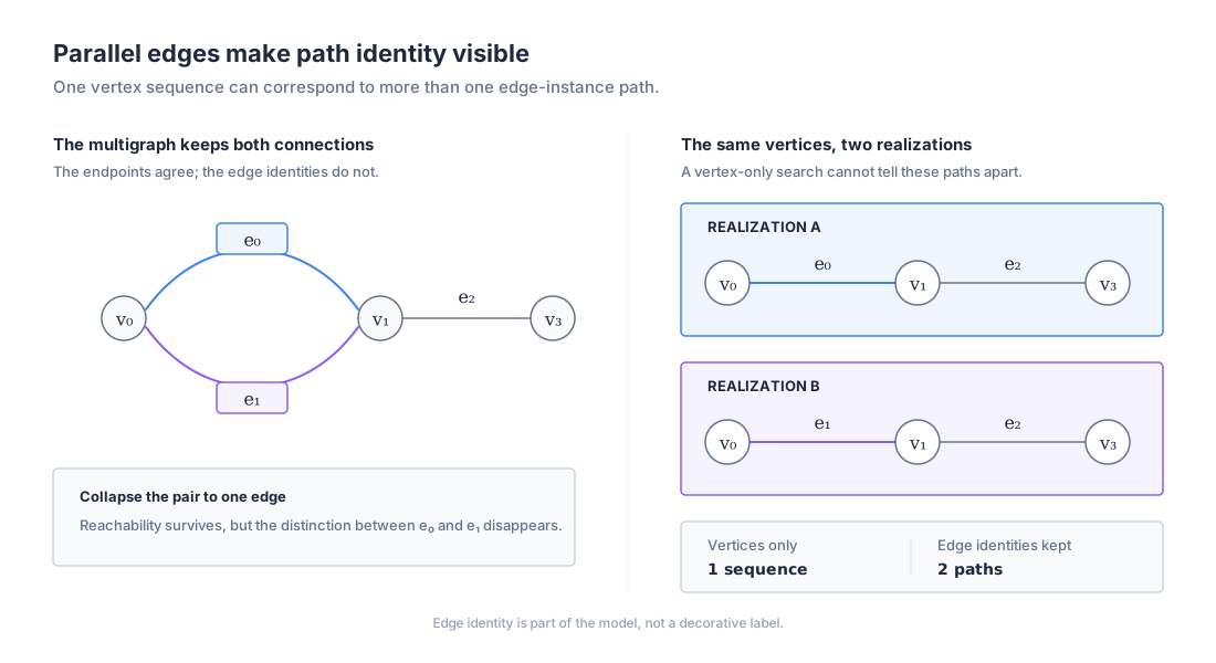 Figure 1: Collapsing parallel edges preserves the vertex sequence but erases the two edge-instance paths that realize it.
We will build the subject from definitions rather than treating parallel edges as an awkward exception.
One verified four-vertex multigraph will accompany us through matrices, shortest paths, cuts, Euler trails, random walks, graph neural networks, and a complete C++23 implementation. Three interactive laboratories expose the same data from different angles. Every major conceptual section ends with five fully solved exercises, for a total of $65$.
Cover the solutions and try each problem first: the article then becomes a compact course rather than a passive tour. Like everything on this blog, this article was created for you to learn, not for you to read. There is a difference. Understand this difference and win.
1. Why one edge is sometimes not enough
A simple graph permits at most one undirected edge ${u,v}$ for each unordered pair of distinct vertices. That model answers questions such as can $u$ reach $v$? efficiently, but it asserts that all direct connections between the pair can be represented by one fact. Real systems frequently violate that assertion.
Consider a transport network. Two bridges may connect the same banks, or two bus services may connect the same stops. The endpoints agree, but the bridge identities, capacities, tolls, and failure modes do not. In an airline network, morning and evening flights connect the same airports while carrying different departure times, fares, and aircraft. In a financial ledger, each transfer is an event with its own amount and timestamp. In a communication network, parallel physical links increase available bandwidth and provide redundancy. Collapsing these edges into one unweighted edge preserves only the weakest statement: some connection exists. The weakest statement rarely describes or solves the problem.
We can sometimes aggregate parallel edges, but aggregation is a modeling decision, not a harmless preprocessing step. Summing capacities may be correct for a maximum-flow problem. Taking the minimum travel time may be correct for a shortest-route problem when departures do not matter. Counting transfers may be a useful feature for fraud detection. None of these summaries is universally interchangeable with the original edge set. None of these sets represents the real problem. All of them simplify the model and lose the nuances of the real world.
The decisive question is not does the software support multigraphs? It is which distinctions must the answer preserve? If an edge has an identity, state, capacity, time, relation type, or failure event that matters independently, the representation should keep it independently.
At this point, we abandon the mathematical concepts covered in undergraduate studies and enter the waters of pure research and advanced mathematics. Courage, from this point forward, will be your best companion.
1.1 A modeling test before the first algorithm
Determining when a simple graph fails requires more than theoretical definitions. The choice of representation dictates what information survives the transition from the real world to the data structure. We need an empirical test to verify if aggregating connections destroys the independent attributes the system is designed to analyze.
We can make the decision operational.
Imagine removing one connection while leaving another connection with the same endpoints intact. If the application can observe that state, the two connections are different edge instances. Imagine permuting their attributes. If the answer changes, those attributes cannot be compressed into an endpoint-level Boolean. Finally, imagine replacing the complete bundle by a summary. We should be able to name an invariant that the summary preserves.
For reachability, the invariant is simply whether multiplicity is zero or positive. For total simultaneous capacity, the invariant may be the sum of capacities. For the cheapest static direct move, it may be the minimum cost. For independent reliability, neither the sum nor the minimum is enough: we need the probability and dependence structure of each failure. For a scheduled service, a set of time intervals or events may be the smallest honest summary.
This test also protects us from overmodeling. Suppose five observations all report the same permanent relationship and carry no independent identity. Five parallel edges would incorrectly amplify the relationship in degree, random-walk, and message-passing calculations. Duplicate database rows are not automatically parallel edges. An edge instance should correspond to a meaningful instance in the domain, not merely to the number of times a collector happened to copy the same fact.
The distinction between evidence and ontology is especially important in learned systems. Here, an ontology is the model’s account of what kinds of entities, relations, and events exist in the domain, together with the identity rules that determine when two records describe the same thing. It tells us, for example, whether works_for denotes one persistent relationship between a person and a company, whether every payment is a separate event, and whether a timestamp belongs to the relationship itself or to an observation of it. Evidence, by contrast, is what a sensor, database, annotator, or experiment has recorded in support of those ontological claims. Repeated evidence does not automatically imply repeated objects.
Ten independent observations that the same person works for the same company may strengthen our confidence in one relationship. Encoding them as ten parallel edges would instead assert that ten relationship instances exist, causing the observation count to amplify degrees, random-walk probabilities, and message-passing contributions. One edge with confidence, provenance, or observation-count features may therefore be the honest representation. Ten transfers between two accounts are different: each transfer usually has its own amount, timestamp, identifier, and causal role, so the ten records describe ten ontological events and often require ten timestamped edges. Graph construction therefore does more than prepare input. It decides which objects the learner is allowed to distinguish and embeds assumptions about identity, independence, multiplicity, and sufficient summaries before any model parameter is estimated.
1.2 Solved exercises
Exercise 1.1. Choose a graph model. Two cities are connected by a highway and a railway. We want to plan closures independently. Should we use a simple graph or a multigraph?
Solution. We need a multigraph with two edge instances because the closures are independent events. A single edge labeled “connected” would make it impossible to close the railway while leaving the highway available.
Exercise 1.2. Find a safe aggregation. Three parallel communication links have capacities $4$, $7$, and $9$ Gb/s and can carry traffic simultaneously. What single capacity preserves their contribution to a maximum-flow calculation?
Solution. Their capacities add, so the aggregate capacity is $4+7+9=20$ Gb/s. This aggregation preserves the cut capacity for that pair, but it does not preserve which individual link fails.
Exercise 1.3. Reject a misleading aggregation. Two flights join the same airports, one at 08:00 and one at 20:00. Why is the minimum flight duration alone insufficient for itinerary planning?
Solution. Feasible connections depend on departure and arrival times, not only duration. The faster flight may leave before a passenger arrives, so replacing both events by one minimum-duration edge can manufacture an impossible itinerary.
Exercise 1.4. Distinguish repeated observations from weight. Ten transfers occur from account $u$ to account $v$. When is one weighted edge of weight $10$ inadequate?
Solution. It is inadequate when amounts, timestamps, currencies, or transaction identifiers affect the task. The weight preserves a count, but it erases the event sequence and every per-transfer attribute.
Exercise 1.5. Decide what a simple graph still preserves. If every nonempty bundle of parallel edges is replaced by one edge, which property is certainly preserved: reachability, total capacity, or the number of routes?
Solution. Reachability is preserved because a pair remains adjacent exactly when at least one edge existed. Total capacity and edge-distinct route counts generally change.
2. Definitions: multiplicity, identity, loops, and degree
An undirected multigraph is conveniently defined as a triple
\[G=(V,E,\partial),\]where $V$ is a finite vertex set, $E$ is a finite set of edge instances, and $\partial:E\to{{u,v}:u,v\in V}$ maps each edge to its unordered pair of endpoints. Distinct elements of $E$ may have the same image under $\partial$. Thus $e_a\ne e_b$ can coexist while $\partial(e_a)=\partial(e_b)={u,v}$. Figure 2 makes the role of $\partial$ concrete for our recurring graph: it assigns endpoints to edge instances without identifying distinct edges that receive the same pair.
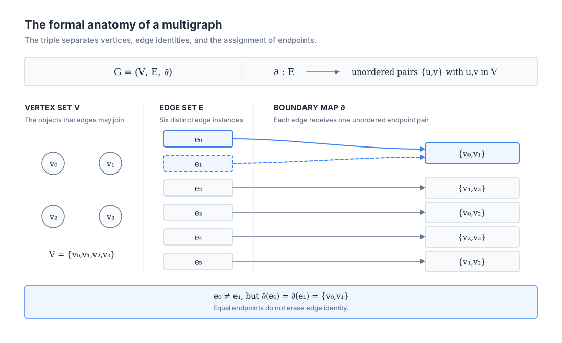 Figure 2: The boundary map assigns both distinct edge instances $e_0$ and $e_1$ to $\lbrace v_0,v_1\rbrace$, so equality of endpoints does not erase edge identity.
The multiplicity
\[\mu(u,v)=\left|\{e\in E:\partial(e)=\{u,v\}\}\right|\]counts the edges between $u$ and $v$. A simple graph, which we use to learn, is the special case in which $\mu(u,v)\in{0,1}$ for distinct vertices and no edge joins a vertex to itself. Terminology varies: many authors allow a multigraph to contain parallel edges but not loops, and call a graph that also allows loops a pseudograph. We will state explicitly when loops are permitted instead of relying on the name.
An edge identifier is not a cosmetic label. If $e_0$ and $e_1$ share endpoints, they remain different members of $E$. Algorithms for trails, capacities, failures, temporal events, and edge prediction need that identity. A data structure that stores only neighbouring vertex numbers cannot reconstruct it.
For a loopless undirected multigraph,
\[\deg(v)=\sum_{u\in V}\mu(u,v).\]If loops are allowed, each loop contributes $2$ to the undirected degree. This convention preserves the handshake theorem:
\[\sum_{v\in V}\deg(v)=2|E|.\]Our recurring graph has vertices $V={v_0,v_1,v_2,v_3}$ and six edge instances:
\[\begin{aligned} e_0&=\{v_0,v_1\},& e_1&=\{v_0,v_1\},& e_2&=\{v_1,v_3\},\\ e_3&=\{v_0,v_2\},& e_4&=\{v_2,v_3\},& e_5&=\{v_1,v_2\}. \end{aligned}\]| Only $e_0$ and $e_1$ are parallel. The degree sequence is $(3,4,3,2)$, whose sum $12$ equals $2 | E | =12$. |
The Handshake Theorem
The theorem is based on the principle that every undirected edge connects exactly two endpoints. Following the real-world analogy, every handshake involves two hands, meaning the sum of all hands shaken will always be twice the total number of handshakes.
Beyond preserving the formula, this theorem is used to:
- Prove that any undirected graph must contain an even number of vertices with an odd degree.
- Serve as a strict invariant to validate degree sequences when constructing and testing graph data structures.
- Guarantee consistency in dynamic graphs, ensuring that adding or removing edges always keeps the total degree sum even.
2.1 Directed edges and maps between graph classes
For a directed multigraph, the endpoint map becomes
\[\partial:E\to V\times V.\]The ordered pair matters. We write $\mu(u,v)$ for the number of arcs directed from $u$ to $v$, and it need not equal $\mu(v,u)$. The out-degree and in-degree are
\[\deg^+(u)=\sum_{v\in V}\mu(u,v), \qquad \deg^-(u)=\sum_{v\in V}\mu(v,u).\]Every arc contributes one to a source out-degree and one to a destination in-degree, so
\[\sum_{v\in V}\deg^+(v)=|E|=\sum_{v\in V}\deg^-(v).\]Several common conversions are worth naming because each discards information. The underlying simple graph replaces every positive multiplicity by one and, for a directed graph, may also forget orientation. A weighted projection applies a reducer to each parallel bundle. The support graph keeps an edge precisely where multiplicity is positive. Conversely, expanding an integer-weighted edge of weight $k$ into $k$ unit parallel edges is valid only when the weight really denotes $k$ exchangeable units. A distance of $k$ kilometers is not $k$ parallel roads.
Figure 3 follows one three-arc directed multigraph through these conversions. The support projection preserves both directions but discards edge identity and multiplicity; the weighted projection retains direction and counts but still cannot recover the original edge identities. Forgetting orientation removes yet another distinction.
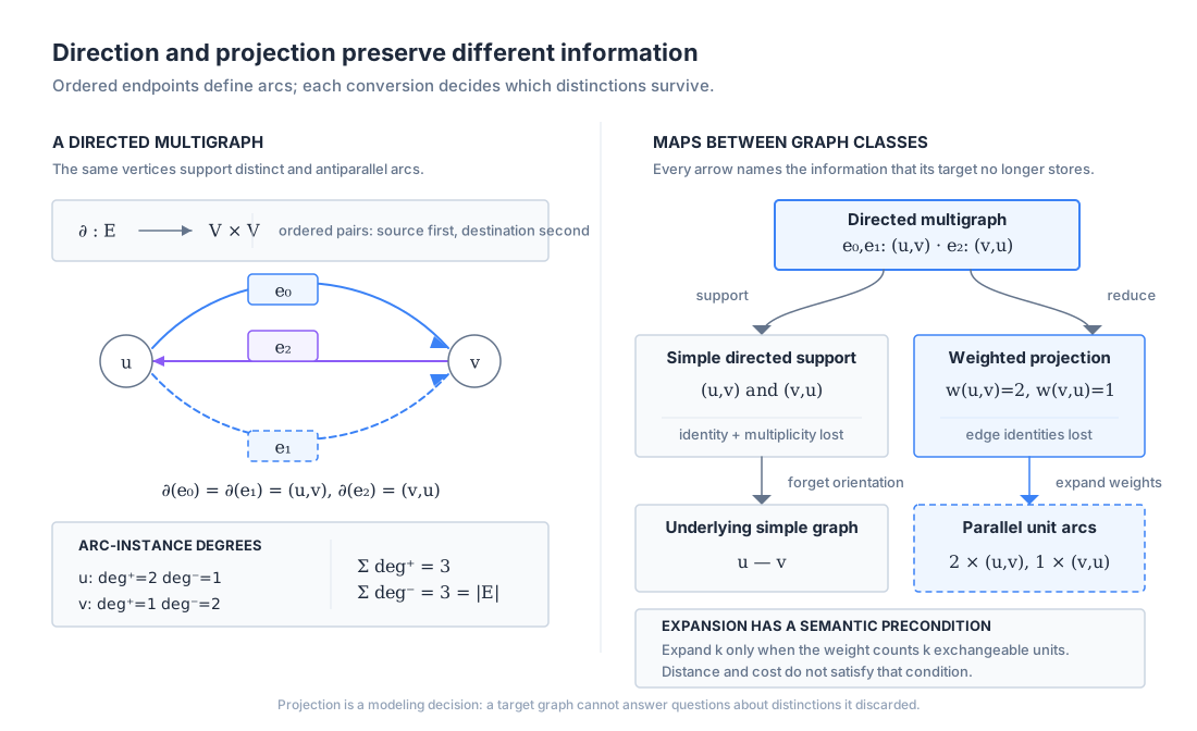 Figure 3: Direction, multiplicity, and edge identity survive different projections; expanding a weight back into parallel arcs is valid only when that weight counts exchangeable units.
Graph isomorphism also respects edge multiplicity. A bijection $f:V(G)\to V(H)$ is a multigraph isomorphism when
\[\mu_G(u,v)=\mu_H(f(u),f(v))\]for every endpoint pair, with direction preserved in a directed graph. Edge attributes impose further preservation conditions. Two pictures with the same support graph can therefore represent nonisomorphic multigraphs.
2.2 Solved exercises
Exercise 2.1. Compute multiplicities. Find $\mu(v_0,v_1)$, $\mu(v_1,v_2)$, and $\mu(v_0,v_3)$ in the recurring graph.
Solution. The values are $2$, $1$, and $0$, respectively. Edges $e_0,e_1$ form the first bundle, $e_5$ forms the second, and no direct edge joins $v_0$ to $v_3$.
Exercise 2.2. Verify the degree sequence. Compute $\deg(v_1)$ from edge identities.
Solution. Edges $e_0,e_1,e_2,e_5$ are incident to $v_1$, so $\deg(v_1)=4$. Counting distinct neighboring vertices would give only $3$ and would not be the multigraph degree.
Exercise 2.3. Add a loop. Add one loop $e_6$ at $v_3$. What becomes of $\deg(v_3)$ and the total degree sum?
| Solution. The loop contributes $2$, so $\deg(v_3)$ rises from $2$ to $4$. The degree sum rises from $12$ to $14$, matching $2 | E | =2\cdot7$. |
Exercise 2.4. Recover the edge count. A loopless undirected multigraph has degree sequence $(5,5,2,2)$. How many edge instances does it contain?
| Solution. The sum is $14$. By the handshake theorem, $2 | E | =14$, so $ | E | =7$. |
| Exercise 2.5. Separate degree from neighborhood size. What are $\deg(v_0)$ and $ | \mathcal N(v_0) | $ in the recurring graph? |
| Solution. Vertex $v_0$ has three incident edges, $e_0,e_1,e_3$, so $\deg(v_0)=3$. Its distinct-neighbor set is ${v_1,v_2}$, so $ | \mathcal N(v_0) | =2$. |
3. Representations that preserve parallel edges
The most direct representation is an edge table with one row per edge instance. The recurring graph needs six rows, even though only five unordered endpoint pairs are occupied. Per-edge attributes such as capacity, timestamp, relation type, and cost belong in those rows.
An adjacency list must also preserve identity. Instead of storing only neighbor $v$, each incidence stores a pair (neighbor, edge_id). An undirected non-loop edge appears in two adjacency lists but remains one edge instance in the edge table. This separation prevents an algorithm from confusing two incidences with two edges.
The adjacency matrix of a loopless multigraph records multiplicity:
\[A_{ij}=\mu(v_i,v_j).\]For our graph,
\[A=\begin{bmatrix} 0&2&1&0\\ 2&0&1&1\\ 1&1&0&1\\ 0&1&1&0 \end{bmatrix}, \qquad D=\operatorname{diag}(3,4,3,2).\]The row sum of $A$ is the degree when there are no loops. With loops, conventions for $A_{ii}$ differ, so an implementation must document whether a loop contributes $1$ or $2$ on the diagonal and compute degree consistently.
| The incidence matrix $B\in{0,1}^{ | V | \times | E | }$ gives every edge its own column: |
Columns $0$ and $1$ are equal because $e_0$ and $e_1$ have the same endpoints, but they are still separate columns. If we orient each undirected edge arbitrarily and replace the endpoint entries by $-1$ at the tail and $+1$ at the head, we obtain an oriented incidence matrix $C$. Its Laplacian is
\[L=CC^\top=D-A= \begin{bmatrix} 3&-2&-1&0\\ -2&4&-1&-1\\ -1&-1&3&-1\\ 0&-1&-1&2 \end{bmatrix}.\]Parallel edges therefore strengthen the off-diagonal coupling and increase both endpoint degrees. The first laboratory lets us alter multiplicities and watch all three representations change.
3.1 What each representation can and cannot invert
The edge table can reconstruct every structure above when it contains endpoints and identifiers. The multiplicity matrix can reconstruct endpoint counts but cannot recover the original identifiers or attributes. The incidence matrix retains one column per identity, but equal columns reveal only that two edges share endpoints. If column labels are discarded, permuting equal columns makes no mathematical difference, but an external database may still care which column was flight 271 and which was flight 845.
For a directed graph, the oriented incidence matrix has one $-1$ and one $+1$ in every non-loop column. A directed loop produces a zero column under this convention because its tail and head cancel. That is useful algebraically but means the matrix alone cannot detect directed loops. Representation choice must therefore be driven by the queries that must be invertible.
There is also a clean relationship between incidence and adjacency for a loopless undirected multigraph. With the unsigned $0$-$1$ incidence matrix above,
\[BB^\top=D+A.\]The diagonal counts incident edges and the off-diagonal entry counts columns containing both endpoints. With an oriented incidence matrix $C$,
\[CC^\top=D-A=L.\]The arbitrary orientation disappears from the product because reversing a column multiplies it by $-1$, leaving its outer product unchanged. This explains why the Laplacian is naturally a sum of one rank-one contribution per edge instance:
\[L=\sum_{e=\{u,v\}\in E}(\mathbf e_u-\mathbf e_v) (\mathbf e_u-\mathbf e_v)^\top.\]Parallel edges repeat the same rank-one term. They do not require a new spectral theory; they change the coefficient with which a pairwise difference is penalized.
3.2 Solved exercises
Exercise 3.1. Read multiplicity from a matrix. What do $A_{01}=2$ and $A_{03}=0$ mean?
Solution. Exactly two edge instances join $v_0$ and $v_1$, while none joins $v_0$ and $v_3$. Symmetry gives $A_{10}=2$ and $A_{30}=0$.
Exercise 3.2. Verify one Laplacian row. Derive row $0$ of $L$.
Solution. The diagonal is $\deg(v_0)=3$. Off-diagonal entries are negative multiplicities, so the row is $[3,-2,-1,0]$.
Exercise 3.3. Preserve edge attributes. Edges $e_0$ and $e_1$ have costs $4$ and $9$. Can the unweighted multiplicity matrix recover both costs?
Solution. No. It records only that the multiplicity is $2$. We need an edge table or an attribute collection attached to each matrix position.
Exercise 3.4. Check the incidence matrix. Why do columns $0$ and $1$ of $B$ agree without implying $e_0=e_1$?
Solution. A column describes endpoints, and both edges have the same endpoints. Column position is the edge identity, so equal column values do not merge the two elements of $E$.
Exercise 3.5. Measure dense storage. How many entries does a dense multiplicity matrix contain for $10^6$ vertices, regardless of the edge count?
Solution. It contains $10^{12}$ entries. At 8 bytes each that is 8 TB, so sparse edge or compressed-row storage is required for ordinary sparse networks.
4. What does a different path mean?
In casual language, a path is any route. Graph theory needs sharper distinctions. A walk is an alternating sequence
\[v_{i_0},e_{j_1},v_{i_1},\ldots,e_{j_k},v_{i_k}\]in which each edge has the adjacent vertices as endpoints. Vertices and edges may repeat. A trail is a walk with no repeated edge instance. A simple path is a walk with no repeated vertex, apart from the conventional equality of first and last vertex when defining a cycle.
In a simple graph, writing only the vertex sequence determines every traversed edge. In a multigraph it does not. We must state the equivalence relation used to count routes:
- Vertex-sequence distinctness: two paths differ only if their vertex sequences differ.
- Edge-instance distinctness: two paths differ if any traversed edge identifier differs.
- Attribute-distinctness: applications may identify edges by a selected attribute, such as departure time or relation type.
From $v_0$ to $v_3$, our graph has four simple vertex sequences:
\[\begin{aligned} &v_0,v_1,v_3, &&v_0,v_2,v_3,\\ &v_0,v_1,v_2,v_3, &&v_0,v_2,v_1,v_3. \end{aligned}\]The first and third each have two edge-instance realizations because their first step may use $e_0$ or $e_1$. The other two have one realization each. Therefore the same graph contains four vertex-distinct simple paths but six edge-distinct simple paths from $v_0$ to $v_3$.
This is not a contradiction. A count is meaningless until its objects and equality rule are specified. The second laboratory makes that equality rule visible by grouping edge-instance paths under their vertex sequences.
4.1 Equivalence classes and a useful counting formula
We can express the distinction precisely. Let $\mathcal P_E(s,t)$ be the set of edge-instance simple paths. Define $p\sim q$ when their vertex sequences agree. Then the vertex-sequence paths are the equivalence classes $\mathcal P_E(s,t)/{\sim}$. For a fixed simple vertex sequence
\[q=(v_{i_0},v_{i_1},\ldots,v_{i_k}),\]the number of edge-instance realizations is
\[r(q)=\prod_{\ell=1}^{k}\mu(v_{i_{\ell-1}},v_{i_\ell}).\]No edge repeats because the vertex sequence is simple. Therefore
\[|\mathcal P_E(s,t)|= \sum_{q\in\mathcal P_V(s,t)}r(q),\]where $\mathcal P_V$ denotes simple vertex sequences. This identity produces $2+1+2+1=6$ in our graph.
The formula also tells us when projection is safe for enumeration. If every pair on every admissible path has multiplicity one, the two counts agree. If a parallel bundle lies outside the $s$-$t$ path region, it changes neither count. Merely knowing that the graph is a multigraph does not tell us whether a particular query is affected.
Trail counting needs more care. A vertex sequence may repeat a pair, and the choices are no longer independent when the same edge instance cannot be reused. If a route crosses a bundle of size $m$ exactly $r$ times in the same endpoint direction, it has a falling-factor contribution $m(m-1)\cdots(m-r+1)$ when those traversals must use distinct edges. The product-of-multiplicities rule is therefore specific to simple vertex paths, or to walks that permit edge reuse.
4.2 Solved exercises
Exercise 4.1. Classify a route. Is $v_0,e_0,v_1,e_5,v_2,e_3,v_0$ a walk, trail, or simple path?
Solution. It is a trail because the edge instances $e_0,e_5,e_3$ are distinct. It is not a simple path because $v_0$ repeats.
Exercise 4.2. Count one vertex sequence. How many edge-instance realizations does $v_0,v_1,v_3$ have?
Solution. The first step can use $e_0$ or $e_1$, while the second must use $e_2$. The product is $2\cdot1=2$ realizations.
Exercise 4.3. Generalize the product rule. A vertex sequence traverses endpoint pairs whose multiplicities are $3$, $2$, and $4$. How many edge-instance realizations does it have?
Solution. Choices at the three steps are independent, so the count is $3\cdot2\cdot4=24$. This assumes edge reuse is not otherwise prohibited by the chosen route.
Exercise 4.4. Explain why infinity appears. If walks rather than simple paths are counted in a graph containing a reachable cycle, why may the number of routes be infinite?
Solution. We can traverse the cycle zero, one, two, or any finite number of times before continuing to the destination. Each repetition yields another walk.
Exercise 4.5. State an API contract. A function is named count_paths(source, target). What two missing choices make the name unsafe?
Solution. It must specify the allowed object, such as walk, trail, or simple path, and the equality rule, such as vertex sequence or edge-instance sequence. Without both, callers cannot interpret the result.
5. Shortest paths and their multiplicity
For an unweighted multigraph, the distance $d(s,t)$ is still the minimum number of edges in a path from $s$ to $t$. Parallel unit edges do not reduce distance: two direct edges from $u$ to $v$ both have length one. They do, however, change the number of shortest edge-instance paths.
| A breadth-first search, or BFS, computes distances in $O( | V | + | E | )$ time when every edge instance is scanned once. To count shortest edge-instance paths, maintain ways[v] together with distance[v]. Initialize ways[s]=1. When scanning an incidence $u\to v$: |
Each parallel incidence performs the addition separately. In our graph, $d(v_0,v_3)=2$. There are two shortest vertex sequences, through $v_1$ and through $v_2$, but three shortest edge-instance paths: $(e_0,e_2)$, $(e_1,e_2)$, and $(e_3,e_4)$.
5.1 Why the counting recurrence is correct
BFS partitions reachable vertices into layers $L_k={v:d(s,v)=k}$. Every shortest path to a vertex in $L_{k+1}$ ends with an edge instance from some predecessor in $L_k$. It cannot arrive from an earlier layer because that would give a shorter distance, and an arrival from the same or later layer would not be shortest. The sets of paths grouped by their final edge instance are disjoint. Adding ways[u] once for every eligible incidence $u\to v$ therefore counts every shortest edge-instance path exactly once.
The discovery branch and equal-distance branch must remain distinct. On first discovery, ways[v] receives the count from the first predecessor and $v$ enters the queue. Later predecessors in the same BFS layer add their counts without re-enqueuing $v$. An incidence leading to a vertex at a smaller distance is ignored for counting because it cannot be the final step of a shortest route.
To count vertex sequences instead, we should not simply deduplicate each adjacency list if edges carry weights or state. For an unweighted static query, grouping incidences by neighbor during the recurrence is sufficient because each predecessor vertex should contribute once. A more general implementation needs a bundle-level rule that decides whether any edge in the bundle realizes the current optimum and how equivalent realizations are grouped.
Weighted parallel edges require an explicit policy. Dijkstra’s algorithm can scan all edge instances and naturally select the cheapest realizations when weights are nonnegative. If edges are collapsed first, using the minimum weight preserves shortest distance between endpoints in a static graph, but it does not preserve the number of equally shortest edge-instance paths unless we also preserve how many edges attain that minimum. Timetabled and state-dependent edges generally cannot be reduced to one scalar this way.
Path counts grow quickly. Even a layered acyclic multigraph can have exponentially many paths, so std::uint64_t may overflow. Production code should either use arbitrary-precision integers, count modulo a documented modulus, or detect overflow.
For negative weights, Dijkstra’s assumption fails just as it does in a simple graph. Bellman-Ford can scan every edge instance, but a pair of antiparallel negative arcs or a negative cycle makes shortest walks undefined because cost can decrease without bound. Again, “path” must be distinguished from “walk”: a minimum over finitely many simple paths may exist even when no minimum-cost walk exists, but finding it under general constraints is a different problem.
5.2 Solved exercises
Exercise 5.1. Count shortest routes. Give the shortest distance, vertex-sequence count, and edge-instance count from $v_0$ to $v_3$.
Solution. The distance is $2$. There are two shortest vertex sequences, $v_0,v_1,v_3$ and $v_0,v_2,v_3$, and three edge-instance realizations.
Exercise 5.2. Increase one multiplicity. Add a third edge between $v_0$ and $v_1$. What changes in Exercise 5.1?
Solution. Distance remains $2$ and the vertex-sequence count remains $2$. The route through $v_1$ now has three realizations, so the edge-instance count rises to $3+1=4$.
Exercise 5.3. Collapse weighted edges carefully. Parallel edges from $u$ to $v$ have weights $2,2,5$. Which summary preserves shortest distance, and what additional value preserves the count of cheapest direct choices?
Solution. Store minimum weight $2$. Also store that two edge instances attain the minimum; otherwise a shortest-path counter would report one direct realization instead of two.
Exercise 5.4. Apply the BFS recurrence. When processing $u$, suppose $d(u)=3$, $\mathrm{ways}(u)=5$, $d(v)=4$, and one more parallel incidence $u\to v$ is scanned. What happens?
Solution. Since $d(v)=d(u)+1$, add the five routes ending at $u$. Thus $\mathrm{ways}(v)$ increases by $5$ without changing its distance.
Exercise 5.5. Bound path-count growth. A chain has ten stages, with three parallel edges at every stage. How many edge-instance paths connect its endpoints?
Solution. Every stage offers three independent choices, so the count is $3^{10}=59{,}049$. The vertex sequence is unique.
6. Edge-disjoint paths, cuts, and maximum flow
Parallel edges model redundancy only if we ask a question that preserves their independence. Two $s$-$t$ paths are edge-disjoint when they share no edge instance, although they may share vertices. The local edge connectivity $\lambda(s,t)$ is the maximum number of pairwise edge-disjoint $s$-$t$ paths.
An $s$-$t$ edge cut is a set of edges whose removal disconnects $s$ from $t$. Menger’s edge theorem states that, for distinct vertices in a finite graph, the maximum number of pairwise edge-disjoint $s$-$t$ paths equals the minimum size of an $s$-$t$ edge cut. Parallel edges count separately on both sides of this equality.
In the recurring graph, the paths $v_0,e_0,v_1,e_2,v_3$ and $v_0,e_3,v_2,e_4,v_3$ are edge-disjoint. No third path can exist because only $e_2$ and $e_4$ enter $v_3$; removing those two edges disconnects it. Therefore
\[\lambda(v_0,v_3)=2.\]The algorithmic version assigns capacity $1$ to every edge instance and computes maximum flow. The integral-flow property decomposes a maximum flow of value $k$ into $k$ edge-disjoint paths. For an undirected edge, a careful implementation uses an undirected-capacity construction rather than accidentally allowing one unit independently in each direction. With arbitrary capacities, parallel edges may either remain separate or be summed when only total flow matters.
Edge-disjointness differs from vertex-disjointness. The two paths above share only their endpoints, so they satisfy both notions. In another graph, two routes may use different edges through the same intermediate router. They survive one link failure but not that router’s failure.
6.1 Why packing and cutting meet
The easy half of Menger’s equality is weak duality. Every $s$-$t$ path must cross every $s$-$t$ cut. If paths are edge-disjoint, each needs a different cut edge, so the size of any path packing is at most the size of any cut. In symbols,
\[\max\{\text{edge-disjoint paths}\} \le \min\{\text{edge-cut size}\}.\]The substantive half proves that some packing reaches the minimum cut. Unit-capacity maximum flow provides an algorithmic proof. Because all capacities are integers, an augmenting-path algorithm maintains an integral flow. A positive integral unit on an edge can be decomposed into source-to-destination paths, after removing any flow cycles. No edge instance carries more than one unit, so those paths are edge-disjoint.
Undirected capacity deserves a precise contract. Replacing an undirected unit edge by two unrelated directed unit arcs permits simultaneous one-unit flows in opposite directions. That does not represent one shared physical link in all formulations. One safe construction introduces a capacity gadget that limits their combined use, while another algorithm works directly with skew-symmetric undirected flow. For the single-source single-sink maximum value, antiparallel flow can often be cancelled, but relying on that fact without stating the model is fragile when flows are later decomposed or extended.
Vertex-disjoint paths reduce to edge capacity by splitting each intermediate vertex $v$ into $v_{\text{in}}$ and $v_{\text{out}}$ connected by a unit-capacity arc. Incoming edges terminate at the first copy and outgoing edges leave the second. The split arc becomes the resource that at most one route may consume. Source and destination receive unbounded or sufficiently large split capacity.
The flow laboratory lets us vary a parallel bundle and compare the visible routes with the bottleneck cut.
6.2 Solved exercises
Exercise 6.1. Exhibit a maximum packing. Name two edge-disjoint paths from $v_0$ to $v_3$.
Solution. Use $(e_0,e_2)$ through $v_1$ and $(e_3,e_4)$ through $v_2$. Their edge sets are disjoint.
Exercise 6.2. Certify optimality. Which two-edge cut proves that a third edge-disjoint route cannot exist?
Solution. Remove ${e_2,e_4}$, the complete set of edges incident to $v_3$. The destination becomes isolated, so every $v_0$-$v_3$ path used one of those two edges.
Exercise 6.3. Distinguish two failure models. Two edge-disjoint routes share intermediate vertex $x$. What failure do they tolerate, and what failure defeats both?
Solution. They tolerate the loss of any one edge because the other path uses different edge instances. Failure of vertex $x$ disables both routes, so they are not internally vertex-disjoint.
Exercise 6.4. Read a flow value. Five parallel unit-capacity edges are the only connections crossing an $s$-$t$ cut. What upper bound does the cut impose?
Solution. Its capacity is $5$, so every $s$-$t$ flow has value at most $5$. If five disjoint routes reach those edges on both sides, the bound is attained.
Exercise 6.5. Aggregate capacities. Parallel edges have capacities $3$, $4$, and $8$. If individual failures and path identities do not matter, what capacity can replace the bundle?
Solution. A single capacity-$15$ edge preserves all cut and maximum-flow values. It does not preserve a decomposition into physical edge instances.
7. Euler trails: use every edge exactly once
An Euler problem asks us to traverse edge instances, not merely endpoint pairs. An Euler trail uses every edge exactly once. An Euler circuit is an Euler trail that returns to its starting vertex. Parallel edges pose no theoretical difficulty because each has its own identity; they expose the inadequacy of an adjacency structure that discarded those identities.
For a finite connected undirected multigraph after isolated vertices are ignored:
- an Euler circuit exists exactly when every vertex has even degree;
- an open Euler trail exists exactly when two vertices have odd degree, and its endpoints must be those vertices.
Loops contribute $2$ to degree and can be traversed once. In our graph, the degrees are $(3,4,3,2)$. The odd vertices are $v_0$ and $v_2$, so no Euler circuit exists, but an Euler trail must run from one of these vertices to the other. One verified trail is
\[v_0,e_3,v_2,e_5,v_1,e_1,v_0,e_0,v_1,e_2,v_3,e_4,v_2.\]Every identifier $e_0,\ldots,e_5$ appears exactly once.
| Hierholzer’s algorithm constructs such a traversal in $O( | V | + | E | )$ time. Starting at a valid endpoint, it follows unused edges until it cannot continue, then splices additional unused-edge circuits into the route. An implementation marks used[edge_id], not used[u][v]. The latter would mark every parallel edge between $u$ and $v$ after traversing only one. |
Euler trails and simple paths answer opposite questions. A simple path prohibits repeated vertices and may ignore most edges. An Euler trail requires every edge once and commonly repeats vertices. Route inspection, street sweeping, and sequencing of assembled fragments often have the Euler form.
7.1 Why the degree criterion and algorithm work
Every time an Euler traversal enters an intermediate vertex along one unused edge, it must leave along another. Incident edges are paired into arrivals and departures, so the degree of an intermediate vertex is even. An open trail has one unpaired departure at its start and one unpaired arrival at its end, making exactly those two degrees odd. A circuit has no endpoints and therefore requires all degrees even.
Parity is necessary but not sufficient if the edge-containing part of the graph is disconnected. Two disjoint cycles give only even degrees, yet no single traversal can jump from one component to the other. The complete theorem therefore requires all vertices of nonzero degree to belong to one connected component.
For sufficiency, begin at an odd vertex for the open case or any non-isolated vertex for the circuit case. Follow unused edges greedily. At any vertex other than the permitted final endpoint, parity prevents us from getting stuck while an unused arrival has brought us there. In the all-even case, the first closed tour may omit edges. If so, connectedness guarantees that a vertex already on the tour is incident to an unused edge. Start another closed tour there and splice it into the first. Repeating this operation is Hierholzer’s construction.
An efficient program keeps a cursor into each adjacency list. Used incidences are skipped, but the cursor never moves backward, so the total scan is linear. The output is commonly built in reverse during stack backtracking. This is why implementations can look unlike the informal “splice circuits” description while enforcing the same invariant.
7.2 Solved exercises
Exercise 7.1. Apply the parity criterion. Why does the recurring graph have an open Euler trail?
Solution. It is connected and exactly two vertices, $v_0$ and $v_2$, have odd degree. The trail must start at one and end at the other.
Exercise 7.2. Verify the displayed trail. How many edges and vertices should any Euler trail of this graph list?
Solution. It lists all $6$ edge instances exactly once and therefore contains $7$ vertex occurrences. The displayed alternating sequence has precisely those lengths.
Exercise 7.3. Add one parallel edge. Add $e_6={v_0,v_2}$. Does an Euler circuit now exist?
Solution. The new edge changes both odd degrees from $3$ to $4$. All four degrees are even and the graph remains connected, so an Euler circuit exists.
Exercise 7.4. Add one loop instead. Add a loop at $v_1$. Does the Euler-trail endpoint set change?
Solution. No. The loop adds $2$ to $\deg(v_1)$, preserving its parity. The only odd vertices remain $v_0$ and $v_2$.
Exercise 7.5. Diagnose a bad marker. Why does a Boolean table used[u][v] fail on $e_0$ and $e_1$?
Solution. Both edges occupy the same table cell. Marking that cell after using $e_0$ falsely marks $e_1$, so the returned route omits an edge instance.
8. A correctness-first C++23 implementation
The implementation below encodes one invariant explicitly: each undirected edge has one stable identifier and two adjacency incidences. The edge table is the source of identity; adjacency is only an index for traversal. Vertices and edge identifiers use distinct strong types so that the compiler rejects accidental substitutions.
The program performs two tasks. A depth-first search enumerates simple paths without repeated vertices while retaining edge identifiers, then reports both equality rules. A BFS computes distance and the number of shortest edge-instance paths. This is a didactic CPU baseline, not a claim of production optimization.
#include <algorithm>
#include <compare>
#include <cstddef>
#include <cstdint>
#include <iostream>
#include <limits>
#include <queue>
#include <set>
#include <stdexcept>
#include <utility>
#include <vector>

struct Vertex {
    std::size_t value{};
    friend constexpr bool operator==(Vertex, Vertex) = default;
    friend constexpr auto operator<=>(Vertex, Vertex) = default;
};

struct EdgeId {
    std::size_t value{};
    friend constexpr bool operator==(EdgeId, EdgeId) = default;
    friend constexpr auto operator<=>(EdgeId, EdgeId) = default;
};

struct Edge {
    Vertex u;
    Vertex v;
};

struct Incidence {
    Vertex neighbor;
    EdgeId edge;
};

class MultiGraph {
public:
    explicit MultiGraph(const std::size_t vertex_count)
        : adjacency_(vertex_count) {}

    [[nodiscard]] std::size_t vertex_count() const noexcept {
        return adjacency_.size();
    }

    [[nodiscard]] EdgeId add_edge(const Vertex u, const Vertex v) {
        require_vertex(u);
        require_vertex(v);
        if (u == v) {
            throw std::invalid_argument("This example expects a loopless graph.");
        }

        const EdgeId id{edges_.size()};
        edges_.push_back(Edge{u, v});

        // One edge identity produces two incidences in an undirected graph.
        adjacency_[u.value].push_back(Incidence{v, id});
        adjacency_[v.value].push_back(Incidence{u, id});
        return id;
    }

    [[nodiscard]] const std::vector<Incidence>& adjacent(
        const Vertex vertex) const {
        require_vertex(vertex);
        return adjacency_[vertex.value];
    }

private:
    void require_vertex(const Vertex vertex) const {
        if (vertex.value >= adjacency_.size()) {
            throw std::out_of_range("Vertex is outside the graph.");
        }
    }

    std::vector<Edge> edges_;
    std::vector<std::vector<Incidence>> adjacency_;
};

struct Path {
    std::vector<Vertex> vertices;
    std::vector<EdgeId> edges;
};

void enumerate_simple_paths(
    const MultiGraph& graph,
    const Vertex current,
    const Vertex target,
    std::vector<bool>& visited,
    Path& active,
    std::vector<Path>& result) {
    if (current == target) {
        result.push_back(active);
        return;
    }

    for (const Incidence incidence : graph.adjacent(current)) {
        if (visited[incidence.neighbor.value]) {
            continue;
        }

        // Vertex visitation defines "simple"; EdgeId preserves parallel choices.
        visited[incidence.neighbor.value] = true;
        active.vertices.push_back(incidence.neighbor);
        active.edges.push_back(incidence.edge);
        enumerate_simple_paths(
            graph, incidence.neighbor, target, visited, active, result);
        active.edges.pop_back();
        active.vertices.pop_back();
        visited[incidence.neighbor.value] = false;
    }
}

struct ShortestPathResult {
    std::size_t distance;
    std::uint64_t edge_instance_count;
};

[[nodiscard]] ShortestPathResult count_shortest_paths(
    const MultiGraph& graph,
    const Vertex source,
    const Vertex target) {
    constexpr std::size_t unreachable =
        std::numeric_limits<std::size_t>::max();
    std::vector<std::size_t> distance(graph.vertex_count(), unreachable);
    std::vector<std::uint64_t> ways(graph.vertex_count(), 0);
    std::queue<Vertex> frontier;

    distance[source.value] = 0;
    ways[source.value] = 1;
    frontier.push(source);

    while (!frontier.empty()) {
        const Vertex current = frontier.front();
        frontier.pop();

        for (const Incidence incidence : graph.adjacent(current)) {
            const std::size_t candidate = distance[current.value] + 1;
            if (distance[incidence.neighbor.value] == unreachable) {
                distance[incidence.neighbor.value] = candidate;
                ways[incidence.neighbor.value] = ways[current.value];
                frontier.push(incidence.neighbor);
            } else if (distance[incidence.neighbor.value] == candidate) {
                // Every incidence is a separate shortest-path realization.
                ways[incidence.neighbor.value] += ways[current.value];
            }
        }
    }

    return ShortestPathResult{
        distance[target.value], ways[target.value]};
}

int main() {
    MultiGraph graph{4};
    [[maybe_unused]] const EdgeId e0 =
        graph.add_edge(Vertex{0}, Vertex{1});
    [[maybe_unused]] const EdgeId e1 =
        graph.add_edge(Vertex{0}, Vertex{1});
    [[maybe_unused]] const EdgeId e2 =
        graph.add_edge(Vertex{1}, Vertex{3});
    [[maybe_unused]] const EdgeId e3 =
        graph.add_edge(Vertex{0}, Vertex{2});
    [[maybe_unused]] const EdgeId e4 =
        graph.add_edge(Vertex{2}, Vertex{3});
    [[maybe_unused]] const EdgeId e5 =
        graph.add_edge(Vertex{1}, Vertex{2});

    std::vector<bool> visited(graph.vertex_count(), false);
    visited[0] = true;
    Path active{{Vertex{0}}, {}};
    std::vector<Path> paths;
    enumerate_simple_paths(
        graph, Vertex{0}, Vertex{3}, visited, active, paths);

    std::set<std::vector<Vertex>> vertex_sequences;
    for (const Path& path : paths) {
        vertex_sequences.insert(path.vertices);
    }

    const ShortestPathResult shortest =
        count_shortest_paths(graph, Vertex{0}, Vertex{3});

    std::cout << "edge-instance simple paths: " << paths.size() << '\n'
              << "vertex-sequence simple paths: "
              << vertex_sequences.size() << '\n'
              << "shortest distance: " << shortest.distance << '\n'
              << "shortest edge-instance paths: "
              << shortest.edge_instance_count << '\n';
}
Compile with a conforming implementation, for example:
g++ -std=c++23 -O2 -Wall -Wextra -Wpedantic multigraph.cpp -o multigraph
The verified output is:
edge-instance simple paths: 6
vertex-sequence simple paths: 4
shortest distance: 2
shortest edge-instance paths: 3
Enumeration is exponential in the worst case because the number of simple paths is itself exponential. BFS remains linear in the represented graph size. If a count can exceed std::uint64_t, the addition must be checked or replaced by a documented alternative.
8.1 Invariants, tests, and performance boundaries
MultiGraph deliberately does not expose a mutable adjacency vector. If callers could insert an incidence without adding an edge table record, the representation invariant would break. A production class would usually expose edge_count(), edge access, removal semantics, and perhaps stable handles, but those operations should be added around explicit invariants rather than by returning mutable internals.
The nested adjacency vectors are appropriate because graph rows are irregular: each row owns a variable number of incidences. They are not the best final layout for a static graph processed repeatedly. A builder can collect edge records, count degrees, prefix-sum row offsets, and fill flat CSR arrays. The public semantic model stays the same while the execution layout becomes contiguous.
The enumeration DFS marks vertices, not edges, because its contract is simple paths. If we wanted trails, we would instead mark used[edge_id] and permit revisiting vertices. If we wanted walks of bounded length $k$, we would track remaining length and permit both kinds of repetition. A single generic traversal with ambiguous state would be shorter code but a less reliable explanation.
At least five tests belong beside this program:
- the canonical graph produces $(6,4,2,3)$ for the four reported quantities;
- one edge between two vertices produces one path under both equality rules;
- three parallel direct edges produce distance one and three edge-instance shortest paths;
- a disconnected target returns the unreachable sentinel and zero ways;
- invalid vertex insertion throws before mutating either container.
The unreachable sentinel also deserves an API decision. Returning std::size_t::max() is compact for a demonstration, but std::optional<ShortestPathResult> can make absence impossible to confuse with a very large distance. Libraries should choose an interface that makes invalid interpretations difficult.
8.2 Solved exercises
Exercise 8.1. Explain the two incidences. Why does add_edge append twice but return only one identifier?
Solution. An undirected edge can be reached from either endpoint, so adjacency needs two incidences. Both refer to the same physical edge identity and must not be counted as two elements of $E$.
Exercise 8.2. Predict the effect of deduplication. What output changes if every adjacency list is deduplicated by neighbor?
Solution. The two $v_0$-$v_1$ incidences collapse. Edge-instance simple paths fall from $6$ to $4$, and shortest edge-instance paths from $3$ to $2$.
Exercise 8.3. Identify the exponential operation. Which function can take exponential time, and why is that not an implementation accident?
Solution. enumerate_simple_paths can take exponential time because it emits every simple edge-instance path. No algorithm can explicitly output exponentially many objects in polynomial total time.
Exercise 8.4. Check the BFS count type. Why is std::uint64_t safer than std::size_t for a semantic path count but still incomplete?
Solution. It explicitly promises an unsigned 64-bit domain instead of a platform-dependent size type. It still overflows beyond $2^{64}-1$, so the contract needs detection, modular arithmetic, or arbitrary precision.
Exercise 8.5. Add loop support. What must change if loops are accepted?
Solution. add_edge must define whether one or two adjacency incidences represent a loop, and every consuming algorithm must avoid processing the same loop edge twice unintentionally. Degree calculation must still count the loop twice.
9. Random walks, Laplacians, and spanning trees
Multiplicity affects processes even when we never enumerate paths. In the standard random walk on an unweighted multigraph, we choose uniformly among incident edge instances. The transition probability is
\[P_{ij}=\frac{A_{ij}}{\deg(v_i)}.\]From $v_0$, two of the three incident edges lead to $v_1$ and one leads to $v_2$, so $P_{01}=2/3$ and $P_{02}=1/3$. Collapsing the bundle would incorrectly make both probabilities $1/2$. For an undirected connected graph, the stationary distribution is proportional to degree:
\[\pi_i=\frac{\deg(v_i)}{2|E|}.\]Our stationary vector is $(3,4,3,2)/12$.
The combinatorial Laplacian $L=D-A$ treats each parallel edge as another unit of coupling. Its quadratic form makes this explicit:
\[x^\top Lx=\sum_{\{u,v\}\in E}(x_u-x_v)^2.\]The two parallel edges between $v_0$ and $v_1$ contribute the same squared difference twice. The eigenvalues of our verified $L$ are
\[0,\quad 4-\sqrt3,\quad 4,\quad 4+\sqrt3.\]The single zero eigenvalue confirms connectedness.
9.1 From the edge sum to diffusion
The rank-one edge decomposition from Section 3 proves the quadratic identity directly:
\[x^\top Lx = \sum_{e=\{u,v\}} x^\top(\mathbf e_u-\mathbf e_v) (\mathbf e_u-\mathbf e_v)^\top x = \sum_{e=\{u,v\}}(x_u-x_v)^2.\]Thus $L$ is positive semidefinite, and $x^\top Lx=0$ precisely when $x$ is constant across every edge. In a connected graph that means one global constant, giving one zero eigenvector $\mathbf 1$. In a graph with $c$ components, we may choose an independent constant on each component, giving $c$ zero eigenvalues.
The random-walk Laplacian $L_{\mathrm{rw}}=I-D^{-1}A$ connects the same structure to Markov dynamics because $P=D^{-1}A$ is the transition matrix. The symmetric normalized Laplacian
\[L_{\mathrm{sym}}=I-D^{-1/2}AD^{-1/2}\]has real eigenvalues and is similar to $L_{\mathrm{rw}}$ when all degrees are positive. Parallel edges enter through $A$ and $D$ together, so normalization does not simply multiply every effect by the bundle size. It changes relative transition mass.
Multiplicity also changes the number of spanning trees. Kirchhoff’s matrix-tree theorem says that the number of edge-instance spanning trees equals any cofactor of $L$. Deleting row and column $3$ gives a $3\times3$ determinant equal to $13$. Trees that differ only by choosing $e_0$ instead of $e_1$ are different edge-instance trees, as they should be in a reliability model.
For our graph, the cofactor is
\[\det\begin{bmatrix} 3&-2&-1\\ -2&4&-1\\ -1&-1&3 \end{bmatrix} =13.\]The theorem is sensitive to edge identity without any special correction. Each parallel edge contributed its own rank-one term to $L$, and the determinant expansion automatically counts the alternative choices.
9.2 Solved exercises
Exercise 9.1. Compute one transition row. Give all nonzero probabilities from $v_1$.
Solution. Four incident edges leave $v_1$: two to $v_0$, one to $v_2$, and one to $v_3$. Thus $(P_{10},P_{12},P_{13})=(1/2,1/4,1/4)$.
Exercise 9.2. Find the stationary probabilities. What are $\pi_0$ and $\pi_1$?
Solution. Divide degrees by $12$: $\pi_0=3/12=1/4$ and $\pi_1=4/12=1/3$.
Exercise 9.3. Evaluate the quadratic form. Let $x=[1,0,0,0]^\top$. What is $x^\top Lx$?
Solution. Only edges incident to $v_0$ cross from value $1$ to value $0$. There are three such edge instances, so the sum of squared differences is $3$.
Exercise 9.4. Interpret the zero eigenvalue. What would two zero eigenvalues of $L$ indicate?
Solution. The multiplicity of eigenvalue zero equals the number of connected components. Two zeros would indicate two components, independent of how many parallel edges lie inside either component.
Exercise 9.5. Count trees after labeling. If two spanning trees use the same endpoint pairs but one contains $e_0$ and the other $e_1$, are they distinct in the count $13$?
Solution. Yes. A spanning tree is a subset of the edge-instance set $E$, and those subsets differ. Collapsing parallel edges would answer a different counting problem.
10. Message passing and GNNs on multigraphs
A message-passing graph neural network updates a vertex representation by aggregating messages from incident edges:
\[m_i^{(\ell)}= \operatorname{AGG}\left( \left\{ \phi^{(\ell)}\!\left( h_i^{(\ell)},h_j^{(\ell)},a_e \right): e=(j,i)\in E \right\} \right),\] \[h_i^{(\ell+1)} = \psi^{(\ell)}\!\left(h_i^{(\ell)},m_i^{(\ell)}\right).\]The braces denote a multiset indexed by edge instances. If two parallel edges have different attributes $a_{e_0}$ and $a_{e_1}$, they produce two potentially different messages. Even when their attributes agree, a sum aggregator receives the message twice. This is consistent with a multiplicity adjacency matrix: multiplying $AH$ weights a neighboring row by $\mu(i,j)$.
There are three defensible modeling policies:
- Preserve edge instances. Compute one message per edge. Use this for transactions, temporal contacts, reliability, and distinct relation events.
- Aggregate a bundle first. Replace its attributes by a documented sum, mean, minimum, maximum, histogram, or learned set encoding. Use this when only bundle-level behavior matters.
- Project to a simple graph. Keep adjacency and perhaps attach multiplicity as one scalar feature. Use this only when individual edge identity is irrelevant.
These policies are not equivalent. Suppose $h_1=[2,1]$ and two identical edges send $h_1$ to $v_0$. Sum aggregation contributes $[4,2]$, while mean aggregation over the two edges contributes $[2,1]$. A mean over distinct neighbors also gives $[2,1]$, but differs as soon as other neighbors exist because its denominator ignores multiplicity.
10.1 Bundle encoders and symmetry
If a bundle is reduced before vertex aggregation, that reducer should be invariant to the storage order of its edge instances. Let
\[\mathcal E_{ji}=\{a_e:e=(j,i)\in E\}\]be the multiset of attributes on edges from $j$ to $i$. A bundle encoder may take the Deep Sets form
\[b_{ji}=\rho\left(\sum_{a\in\mathcal E_{ji}}\phi(a)\right),\]then a vertex update aggregates messages derived from $(h_j,b_{ji})$. This preserves permutation invariance within the bundle while allowing more information than a fixed sum or mean. It still cannot preserve an order that matters; temporal edges need time-aware sequence or event processing.
There are two nested symmetries. Reordering edge records must not change a graph-level or vertex-level answer, and relabeling vertices should permute vertex outputs consistently. Stable edge identifiers are needed for tracking and supervision, but a model should not learn arbitrary meaning from the numerical value of an ID. IDs select records; attributes carry learnable semantics.
Attention over parallel edges requires the normalization domain to be stated. A softmax over all incoming edge instances makes two identical parallel edges compete separately and jointly receive more mass than one. A softmax over distinct neighbors followed by a bundle encoder answers a different question. Neither is universally correct. The former models events as separate candidates; the latter models neighbors as candidates with structured relationships.
Relation types introduce another axis. An R-GCN uses relation-specific transformations, which is suitable for a knowledge graph containing several typed edges between the same entities. Temporal multigraphs may require messages that depend on timestamps and are ordered or decayed. A standard GCN built from a binary adjacency matrix silently discards both distinctions.
10.2 Solved exercises
Exercise 10.1. Sum parallel messages. Two parallel edges each send $[2,1]$ to $v_0$. What does sum aggregation receive from this bundle?
Solution. It receives $[2,1]+[2,1]=[4,2]$. Multiplicity acts as an integer weight when messages are identical.
Exercise 10.2. Include edge features. Let $\phi(h_j,a_e)=a_eh_j$, $h_j=[2,1]$, and parallel edge weights $a_{e_0}=0.5$, $a_{e_1}=1.5$. What is their summed message?
Solution. The messages are $[1,0.5]$ and $[3,1.5]$. Their sum is $[4,2]$.
Exercise 10.3. Compare two means. Vertex $i$ has two edges to a neighbor with scalar feature $6$ and one edge to a neighbor with feature $0$. Compare the edge mean with the distinct-neighbor mean.
Solution. The edge mean is $(6+6+0)/3=4$. The distinct-neighbor mean is $(6+0)/2=3$, so the choice changes the representation.
Exercise 10.4. Diagnose binary adjacency. What information does setting every positive $A_{ij}$ to $1$ remove?
Solution. It removes multiplicity and makes repeated identical messages indistinguishable from one connection. Any edge-specific attributes already absent from $A$ are also unrecoverable.
Exercise 10.5. Choose a model. A knowledge graph contains works_for and invested_in edges from the same person to the same company. Why is a relation-aware model appropriate?
Solution. The endpoints agree but the semantics differ. Relation-specific messages can transform the two facts differently instead of treating them as duplicate evidence of one relation.
11. Storage, complexity, and execution
| An edge list uses $O( | E | )$ records and is the clearest source of truth. A conventional undirected adjacency list uses $2 | E | $ incidence records, except for whatever loop convention the implementation adopts. Compressed sparse row, or CSR, stores row offsets plus a neighbor array; a multigraph simply retains duplicate neighbor entries. A parallel edge can also carry an aligned edge_id or attribute array. |
Do not call a generic unique operation on CSR rows unless projection to a simple graph is intended. Sorting by neighbor may improve locality and bundle processing, but equal neighbors must remain separate or be reduced by an explicit operator. If edge identity is stable across updates, sorting should move identifiers and attributes together.
The asymptotic costs are expressed in edge instances:
-
BFS, DFS, connected components, and Hierholzer run in $O( V + E )$; -
sparse message passing costs $O( E F)$ for feature width $F$, plus feature transformations; -
building the multiplicity matrix from an edge table costs $O( E )$; - explicit enumeration costs at least the number of objects emitted.
On a CPU, sorting edges by source and destination can expose bundles and improve sequential access. On a GPU, COO or CSR kernels can process one thread or work item per edge instance, then reduce messages by destination. Parallel edges create repeated destination updates, so segmented reduction or carefully chosen atomic accumulation matters. Floating-point summation order can change the last bits; deterministic execution may require a fixed reduction order and usually costs throughput.
Graph libraries differ in their contracts. Some algorithms accept multigraphs natively, some collapse a bundle, and some reject weighted multigraphs because “the weight between two vertices” is ambiguous. The algorithm’s documentation is part of correctness.
11.1 Building CSR without losing identity
Suppose the input is an array of undirected edge records. A two-pass CSR builder first counts one incidence at each endpoint, prefix-sums those counts into row_offsets, and allocates flat arrays neighbors and edge_ids. A second pass writes two aligned entries for every non-loop edge. If loops are supported, the builder applies its declared one-incidence or two-incidence storage convention consistently.
The alignment invariant is
\[\texttt{neighbors}[p]=v \quad\Longleftrightarrow\quad \texttt{edge\_ids}[p]\text{ identifies an edge from the row vertex to }v.\]An optional attribute array indexed by edge ID avoids duplicating large attributes in both incidences. Conversely, storing incidence-specific information, such as orientation relative to the current row, may justify an aligned incidence array.
Dynamic graphs introduce a tradeoff. Flat CSR is compact and cache-friendly but expensive to update in place. Per-vertex vectors or chunked adjacency blocks accept insertions more easily but add allocation and pointer overhead. A common design keeps a mutable edge log, periodically compacts it into CSR, and associates versions or timestamps with snapshots. Stable external IDs must then be mapped to dense internal indices without being silently renumbered.
Parallel bundles create an optimization opportunity when the algorithm allows bundle reduction. Sorted COO records with the same (source,destination) key can be segmented, and attributes can be reduced once before a vertex-level kernel. This changes work from one message per edge to one message per occupied pair only if the chosen reducer is algebraically compatible with the message function. For a nonlinear edge-specific function $\phi(h_j,a_e)$, averaging attributes first is generally not equal to averaging messages afterward.
11.2 Solved exercises
Exercise 11.1. Count incidences. How many adjacency incidences represent our six-edge loopless undirected graph?
Solution. Each edge contributes two incidences, so there are $12$. This equals the degree sum.
Exercise 11.2. Calculate CSR size. With $N$ vertices and $M$ undirected non-loop edges, how many row offsets and neighbor entries are required?
Solution. CSR needs $N+1$ row offsets and $2M$ neighbor entries. Preserving identity adds $2M$ aligned edge identifiers.
Exercise 11.3. Analyze message-passing work. A graph has $M=5\cdot10^6$ edge instances and message width $F=64$. Approximately how many scalar message components are processed?
Solution. The edge stage handles $MF=320\cdot10^6$ scalar components, before counting transformation and reduction overhead.
Exercise 11.4. Find a sorting bug. Neighbors are sorted but the edge-attribute array is not permuted. What fails?
Solution. Attributes become attached to the wrong edge instances. Endpoints may still look valid, making this a silent semantic corruption.
Exercise 11.5. Explain nondeterminism. Why can two GPU runs differ slightly while processing the same parallel messages?
Solution. Concurrent additions may occur in different orders, and floating-point addition is not associative. Fixed-order segmented reduction can improve reproducibility.
12. Failure modes and tests that catch them
Most multigraph bugs are not failures of graph theory. They are silent changes of model.
Loss of edge identity. A map keyed only by (u,v) overwrites earlier edges. Test two parallel edges with different attributes and verify both survive serialization and traversal.
Accidental deduplication. A simple-graph cleanup pass turns multiplicity into a Boolean. Test degree, edge count, and the three shortest edge-instance paths in our canonical graph.
Confused loop degree. One stored loop record is sometimes counted once rather than twice. Test the handshake theorem after adding a loop.
Unstated weighted reduction. Minimum, sum, and mean answer different questions. Name the reducer in the API and test a bundle such as weights $(2,2,5)$.
Double counting undirected edges. Two adjacency incidences are mistaken for two edge instances. Keep a separate edge table and verify that the edge count is half the non-loop incidence count.
Overflow. Path counts wrap to small values while distances remain correct. Use checked arithmetic at the addition point and test a layered multigraph with a known power count.
Unstable identifiers. Deleting or sorting edges changes IDs that external records reference. Decide whether IDs are persistent handles or dense transient indices, then test the declared contract.
| A useful oracle is the canonical example itself. It has $ | E | =6$, degree sequence $(3,4,3,2)$, six edge-distinct simple $v_0$-$v_3$ paths, four vertex sequences, distance $2$, three shortest edge realizations, edge connectivity $2$, an Euler trail from $v_0$ to $v_2$, and $13$ edge-instance spanning trees. A change that alters one of these values needs an explanation. |
12.1 Property-based and metamorphic checks
Example tests catch known errors; properties explore entire input families. Generate small random edge tables, construct adjacency, and verify
\[\sum_v\deg(v)=2|E|\]| for loopless undirected graphs. Verify adjacency symmetry and compare degree with row sums. For every connected small graph, compare the determinant cofactor with a brute-force enumeration of $( | V | -1)$-edge subsets. These tests are slow only on small instances, where they serve as trustworthy oracles. |
Metamorphic tests apply transformations with known effects. Permuting vertex labels must permute adjacency rows and columns without changing path counts or Laplacian eigenvalues. Permuting edge IDs must not change any unlabeled graph result. Duplicating one edge must increase both endpoint degrees by one and add one to the corresponding symmetric adjacency entries. Removing an edge that lies outside every $s$-$t$ route must not change $s$-$t$ distance.
Projection offers another paired test. The support graph must have the same connected components as the multigraph. Unweighted distances must agree because parallel unit edges do not create a shorter endpoint sequence. Edge-instance route counts, random-walk probabilities, degrees, flow capacities, and spanning-tree counts are not expected to agree. A test suite that asserts both the invariants and the intended differences documents the model better than a comment alone.
Finally, serialize and deserialize a graph with two equal-endpoint edges carrying different attributes. Compare edge identities, endpoints, and attributes after the round trip. Many multigraph failures occur at file-format boundaries, after the central algorithms were already tested correctly.
12.2 Solved exercises
Exercise 12.1. Catch an overwritten edge. After inserting $e_0$ and $e_1$, a container reports one item under key (0,1). What representation was probably used?
Solution. A single-value map keyed only by endpoints probably overwrote the first edge. The value should be a collection or the primary key should include an edge identifier.
Exercise 12.2. Detect double counting. The edge table has $6$ rows, but an algorithm reports $12$ undirected edges. What did it likely count?
Solution. It counted adjacency incidences as edge instances. Each non-loop undirected edge appears at both endpoints.
Exercise 12.3. Test overflow. A 41-stage chain has three parallel choices per stage. Does its path count fit in std::uint64_t?
Solution. No. $3^{41}=36{,}472{,}996{,}377{,}170{,}786{,}403$ exceeds $2^{64}-1=18{,}446{,}744{,}073{,}709{,}551{,}615$.
Exercise 12.4. Locate a projection error. Distances pass after deduplication but path counts fail. Why?
Solution. Unit parallel edges do not shorten a route, so reachability and distance can survive projection. Edge-instance multiplicities are exactly what the count needs.
Exercise 12.5. Design a loop test. A graph contains one vertex and three loops. What edge count, degree, and degree sum should a correct undirected implementation report?
| Solution. It reports $3$ edges, degree $6$, and degree sum $6$. The handshake theorem gives $2 | E | =6$. |
13. Directed, temporal, multiplex, and higher-order relatives
A directed multigraph maps each edge to an ordered pair $(u,v)$. Parallel arcs may share direction, while antiparallel arcs $(u,v)$ and $(v,u)$ are different endpoint pairs. In-degree and out-degree count arc instances. Euler conditions become balance conditions: a directed circuit requires equal in-degree and out-degree at every non-isolated vertex plus the appropriate connectivity condition.
A temporal multigraph attaches a timestamp or interval to each edge event. A valid temporal path must respect time order, so a topologically valid vertex sequence may be temporally impossible. Aggregating all events into one static weighted edge destroys causality.
A multiplex or multilayer graph separates relation channels into layers, such as road, rail, and air. It resembles a multigraph but preserves a layer coordinate and often includes interlayer coupling. A labeled multigraph can encode the same raw records, yet multilayer algorithms make layer structure a first-class part of the model.
A line graph turns edge instances into vertices. Parallel edges in the original graph become distinct line-graph vertices with similar neighborhoods, which is useful when the prediction target belongs to edges rather than endpoints. A hypergraph goes in another direction: one hyperedge can join more than two vertices. It should not be simulated by arbitrary collections of parallel pairwise edges when the group interaction itself matters.
The rule remains constant across these extensions: preserve the coordinates on which admissibility and identity depend. Direction, time, layer, endpoint set, and edge identifier are not interchangeable labels.
13.1 Choosing the neighboring formalism
We can choose among these models by asking what makes an event admissible. If only two endpoints and an independent identity matter, use a multigraph. If traversal must respect orientation, use a directed multigraph. If it must also respect chronological order or interval overlap, use a temporal graph. If the relation channel changes transition rules, a multiplex or typed relational graph makes that coordinate explicit. If one event binds a set of three or more entities jointly, use a hypergraph or an incidence-based bipartite representation.
There are useful transformations between the formalisms, but none is free. A temporal projection answers whether contact ever existed, not whether information could travel in time. A multiplex projection answers whether some layer connects two vertices, not whether a permitted sequence of layer transfers exists. A clique expansion of a hyperedge introduces all pairwise links, but it can exaggerate connectivity and loses the identity of the group event.
For edge-centric learning, the line graph is attractive because standard vertex algorithms can act on original edge instances. Two line-graph vertices are adjacent when their original edges share an endpoint. In a multigraph, $e_0$ and $e_1$ share both endpoints but still become two vertices. Care is needed with conventions: an ordinary simple line graph records their adjacency once, while a line multigraph may retain how many endpoints or incidence relationships they share.
These choices also change scale. A clique expansion of a hyperedge of size $k$ creates $\binom{k}{2}$ pairwise edges. A line graph creates one vertex per original edge and can be dense around high-degree hubs. The most semantically direct model may therefore require an algorithm designed for it rather than an expansion that is easier to name but much larger.
13.2 Solved exercises
Exercise 13.1. Count directed degrees. Three parallel arcs go from $u$ to $v$, and one goes from $v$ to $u$. What contributions do they make?
Solution. They add $3$ to $\deg^+(u)$ and $\deg^-(v)$, and $1$ to $\deg^+(v)$ and $\deg^-(u)$. Antiparallel direction is not multiplicity of the same ordered pair.
Exercise 13.2. Check temporal feasibility. Edge $u\to v$ occurs at time $10$ and $v\to w$ at time $8$. Is $u,v,w$ a time-respecting path with nondecreasing times?
Solution. No. The second event occurs before arrival through the first, even though the static projection contains both arcs.
Exercise 13.3. Choose multiplex structure. Road and rail links share endpoints but have separate transfer rules and budgets. Why use layers?
Solution. Layer identity controls costs and admissible transitions. A multiplex model represents both within-layer travel and explicit road-to-rail transfers.
Exercise 13.4. Build a line-graph size. Our recurring multigraph has six edge instances. How many vertices does its line graph have?
Solution. It has six vertices, one for each $e_0,\ldots,e_5$. The parallel pair remains two distinct vertices.
Exercise 13.5. Reject a pairwise replacement. A meeting requires three people to be present simultaneously. Why is a triangle of pairwise edges not always equivalent to one hyperedge?
Solution. The triangle asserts three independent pair relations and can be satisfied pair by pair. The hyperedge represents one irreducible three-way event, so its semantics and algorithms differ.
14. Conclusion
A multigraph is not a simple graph with an inconvenient duplicate. Its edge set contains independent objects, and that identity changes degrees, matrices, random walks, reliability, Euler traversals, path counts, spanning trees, and learned messages. The core discipline is to declare which objects are distinct before choosing an algorithm or representation.
Our four-vertex example made the consequence measurable. It has four simple vertex sequences but six edge-instance simple paths from $v_0$ to $v_3`; two shortest vertex sequences but three shortest edge realizations. Its minimum edge cut has size two, its odd degrees determine an open Euler trail, and its Laplacian counts thirteen edge-instance spanning trees. The C++23 program and laboratories preserve these facts because every edge owns a stable identifier.
Projection and aggregation remain useful. We may sum capacities, minimize costs, count events, or learn a bundle representation. The safe order is always the same: keep the original semantics, state the question, choose a reduction that preserves the required answer, and test it on a graph where multiplicity changes something.
References
- R. Diestel, Graph Theory, 5th ed., Springer, 2017. Author’s book page and sample material.
- K. Menger, “Zur allgemeinen Kurventheorie,” Fundamenta Mathematicae, vol. 10, pp. 96-115, 1927. EuDML record.
- L. R. Ford Jr. and D. R. Fulkerson, “Maximal Flow Through a Network,” Canadian Journal of Mathematics, vol. 8, pp. 399-404, 1956. DOI.
- C. Hierholzer, “Ueber die Möglichkeit, einen Linienzug ohne Wiederholung und ohne Unterbrechung zu umfahren,” Mathematische Annalen, vol. 6, pp. 30-32, 1873. DOI.
- G. Kirchhoff, “Ueber die Auflösung der Gleichungen, auf welche man bei der Untersuchung der linearen Vertheilung galvanischer Ströme geführt wird,” Annalen der Physik und Chemie, vol. 72, pp. 497-508, 1847. Bibliographic record.
- J. Gilmer, S. S. Schoenholz, P. F. Riley, O. Vinyals, and G. E. Dahl, “Neural Message Passing for Quantum Chemistry,” 2017. arXiv:1704.01212.
- M. Schlichtkrull et al., “Modeling Relational Data with Graph Convolutional Networks,” 2017. arXiv:1703.06103.
- NetworkX Developers, “MultiGraph: undirected graphs with self loops and parallel edges.” Official documentation.
- RAPIDS Developers, “Graph algorithm support.” Official cuGraph documentation.
Series Index: Memory in Graphs
- 1. Graph Neural Networks: An Introduction
- 2. Multigraphs: Parallel Edges and Distinct Paths (You are here)
(Updated: )